Data Structures and Algorithms Cheat Sheet
This Data Structures and Algorithms Cheat Sheet was initially by a student of our Master the Coding Interview: Data Structures & Algorithms course.
But we're now sharing it with anyone that wants to learn and remember the key information about data structures & algorithms!
Want to download a PDF version of this Data Structures and Algorithms Cheat Sheet?
Enter your email below and we'll send it to you 👇
Unsubscribe anytime.
If you’ve stumbled across this cheatsheet and are just starting to learn Data Structures and Algorithms, you've made a great choice!
Even if (... when!) you're coding 10 years from now, you'll still be using data structures & algorithms and knowing how and when to use them will make you a better developer.
Data Structures and Algorithms are fundamental concepts in computer science and they're essential for creating efficient and effective software solutions.
Learning and mastering them is a key step to becoming a top 10% Software Engineer or Data Scientist.
Many of the biggest tech companies (Google, Amazon, Meta, etc.) ask data structure & algorithm questions as part of their standard coding interview process for good reason.
That said, if you're currently stuck in an endless cycle of YouTube tutorials and not having success getting hired as a developer at the company of your dreams, ZTM can help.
Come join the Zero To Mastery Academy and take Andrei's Ultimate Coding Interview Bootcamp.
You'll not only learn data structures and algorithms (and Big O) but also the exact steps to take to get more interviews, more job offers, and a higher salary.
Just want the cheatsheet?
Ok, ok we hear you. One last thing before we dive in... if you're interested in this cheat sheet, you'll probably also want to take advantage of our Big O Cheat Sheet as well.
Please enjoy and if you'd like to submit any suggestions, feel free to email us at support@zerotomastery.io
Contents
DATA STRUCTURES CHEAT SHEET:
What are Data Structures?
Arrays
Hash Tables
Linked Lists
Stacks and Queues
Trees
Binary Trees
Graphs
ALGORITHMS CHEAT SHEET:
What is an Algorithm?
Recursion
Stack Overflow
Sorting Algorithms
Bubble Sort
Selection Sort
Insertion Sort
Divide and Conquer
Merge Sort
Quick Sort
Selecting a Sorting Algorithm
Searching Algorithms
Linear Search
Binary Search
BFS
DFS
Selecting a Searching Algorithm
Dijkstra and Bellman-Ford
Negative Edge Weights
Relaxation
Sparse Graphs
Dynamic Programming
Caching
Memoization
Data Structures Cheat Sheet
What are Data Structures?
Data structure is a storage that is used to store and organize data. It is a way of arranging data on a computer so that it can be accessed and updated efficiently. Each data structure is good and is specialized for its own thing.
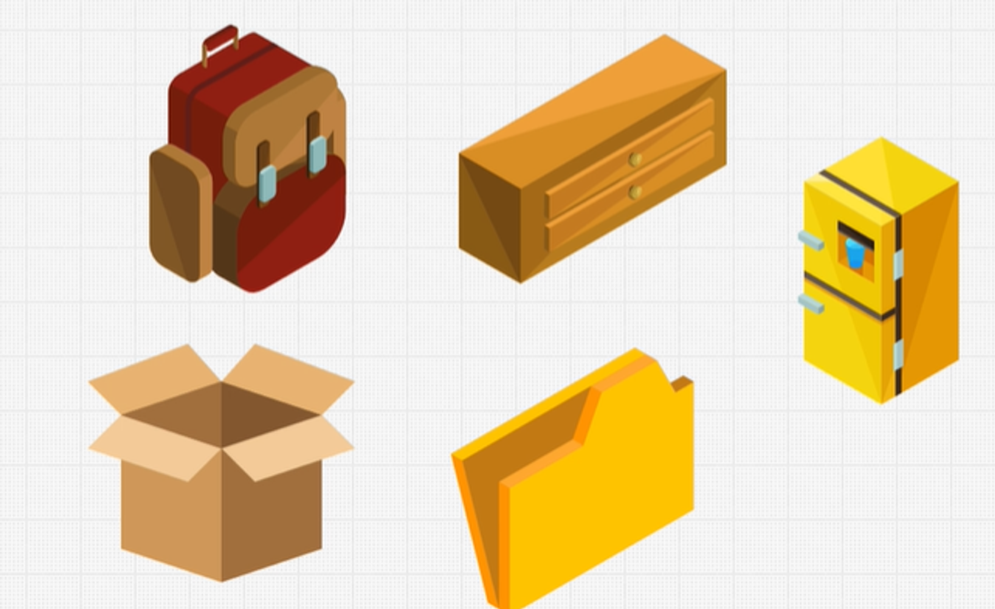
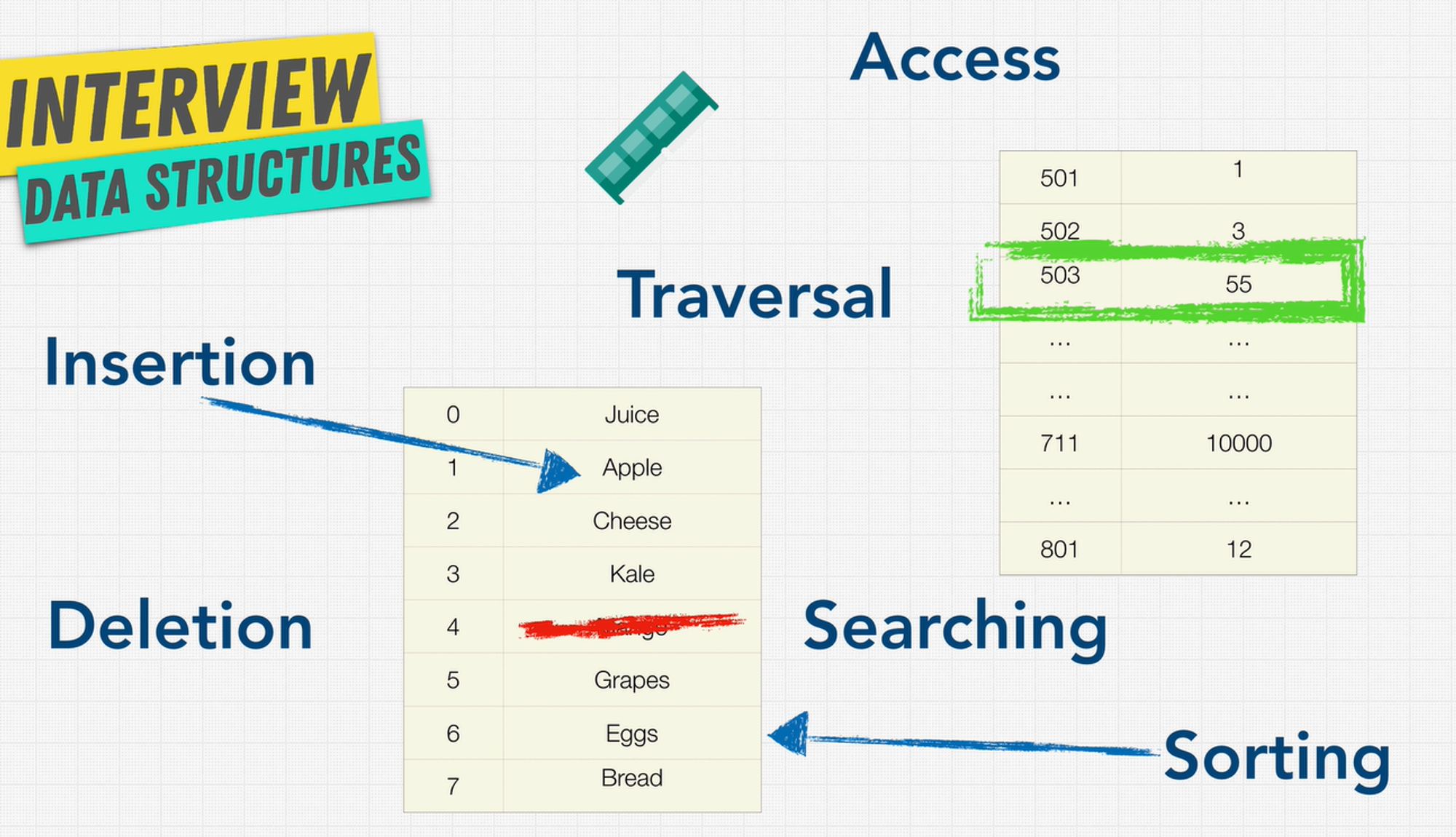
Operations On Data Structures
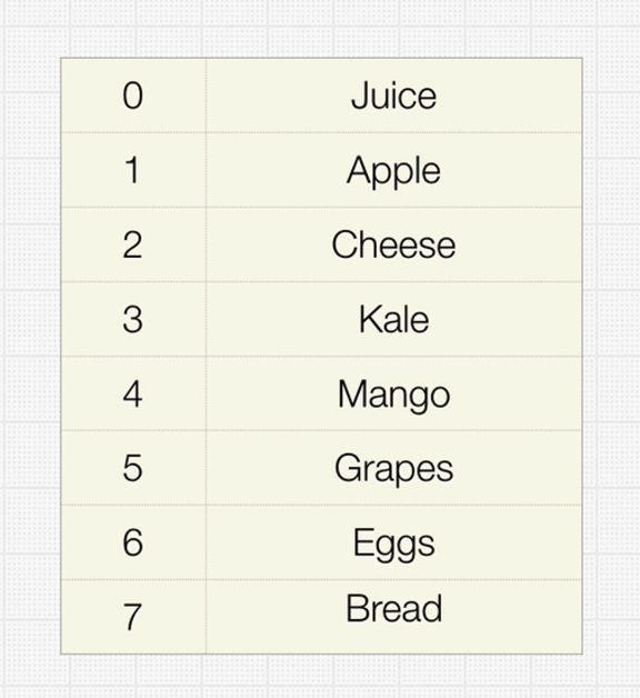
- Insertion: Add a new data item in a given collection of items such as us adding the apple item in memory.
- Deletion: Delete data such as remove mango from our list.
- Traversal: Traversal simply means accessing each data item exactly once so that it can be processed.
- Searching: We want to find out the location of the data item if it exists in a given collection.
- Sorting: Having data that is sorted.
- Access: How do we access this data that we have on our computer?
Arrays
An array is a collection of items of some data type stored at contiguous (one after another) memory locations.
Arrays are probably the simplest and most widely used data structures, and also have the smallest overall footprint of any data structure.
Therefore arrays are your best option if all you need to do is store some data and iterate over it.
Time Complexity
| Algorithm | Average case | Worst case |
|---|---|---|
| Access | O(1) | O(1) |
| Search | O(n) | O(n) |
| Insertion | O(n) | O(n) |
| Deletion | O(n) | O(n) |
The space complexity of an array for the worst case is O(n).
Types of Arrays
Static arrays:
- The size or number of elements in static arrays is fixed. (After an array is created and memory space allocated, the size of the array cannot be changed.)
- The array's content can be modified, but the memory space allocated to it remains constant.
Dynamic arrays:
- The size or number of elements in a dynamic array can change. (After an array is created, the size of the array can be changed – the array size can grow or shrink.)
- Dynamic arrays allow elements to be added and removed at the runtime. (The size of the dynamic array can be modified during the operations performed on it.)
When should an Array be used?
Arrays are excellent for quick lookups. Pushing and popping are really quick.
Naturally, having something organized and close to each other in memory speeds up processing because it is organized.
The only drawback is that whenever it's not at the absolute end of the array, we have to shift to race, which makes inserts and deletions take longer.
Finally, it has a fixed size if static arrays are being used.
As a result, you occasionally need to specify how much memory you will need and the size of the array you desire in advance.
However, we can avoid it if we utilize some of the more modern languages that support dynamic arrays.
Arrays Good at 😀:
- Fast lookups
- Fast push/pop
- Ordered
Arrays Bad at 😒:
- Slow inserts
- Slow deletes
- Fixed size* (if using static array)
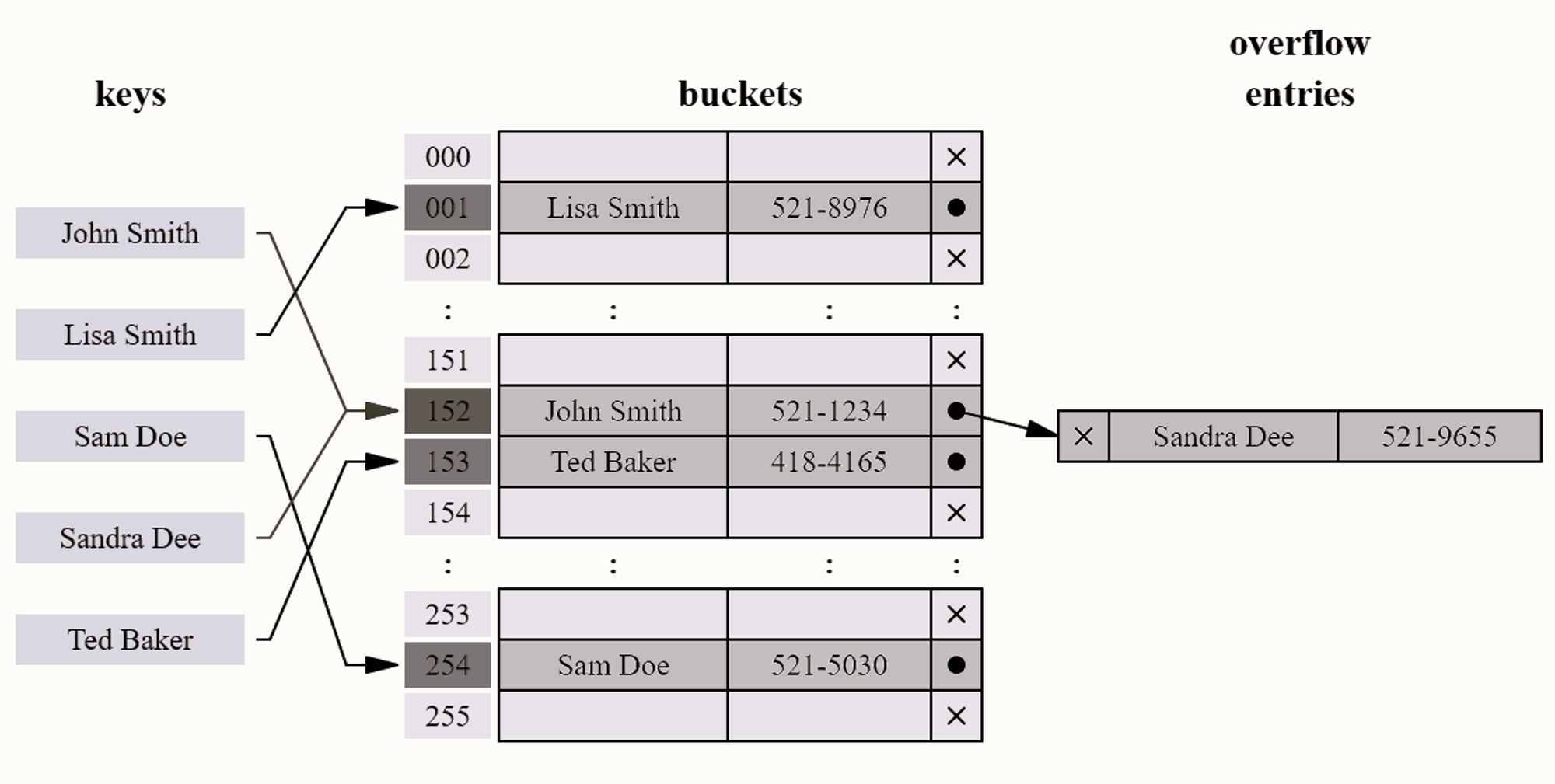
Hash Tables
A hash table is a type of data structure that stores pairs of key-value. The key is sent to a hash function that performs arithmetic operations on it.
The result (commonly called the hash value or hashing) is the index of the key-value pair in the hash table
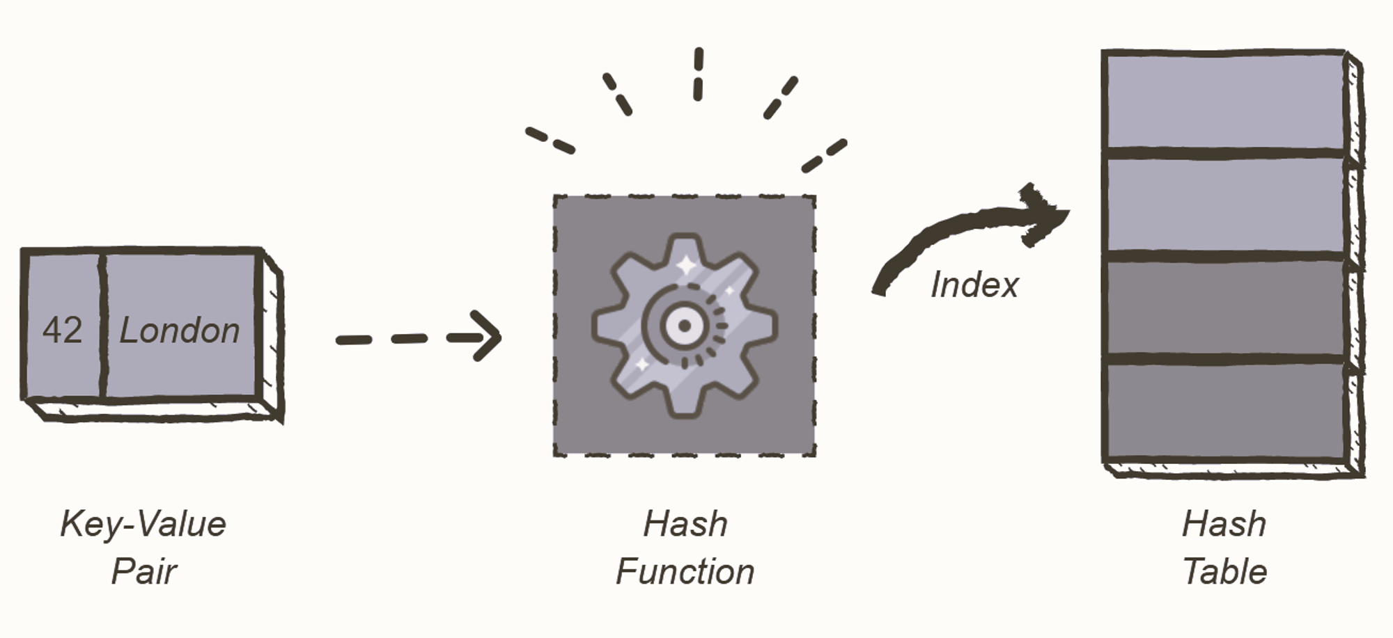
Key-Value
- Key: unique integer that is used for indexing the values.
- Value: data that are associated with keys.
What Does Hash Function Mean?
A hash function takes a group of characters (called a key) and maps it to a value of a certain length (called a hash value or hash). The hash value is representative of the original string of characters, but is normally smaller than the original.
Hashing is done for indexing and locating items in databases because it is easier to find the shorter hash value than the longer string. Hashing is also used in encryption. This term is also known as a hashing algorithm or message digest function.
Collisions
A collision occurs when two keys get mapped to the same index. There are several ways of handling collisions.
Some ways to handle collisions
Linear probing
If a pair is hashed to a slot which is already occupied, it searches linearly for the next free slot in the table.
Chaining
The hash table will be an array of linked lists. All keys mapping to the same index will be stored as linked list nodes at that index.
Resizing the hash table
The size of the hash table can be increased in order to spread the hash entries further apart. A threshold value signifies the percentage of the hash-table that needs to be occupied before resizing.
A hash table with a threshold of 0.6 would resize when 60% of the space is occupied. As a convention, the size of the hash-table is doubled. This can be memory intensive.
When should a Hash Table be used?
Hash tables have incredibly quick lookups, but remember that we need a reliable collision solution; normally, we don't need to worry about this because our language in the computer beneath the hood takes care of it for us.
It allows us to respond quickly, and depending on the type of hash table, such as maps in JavaScript, we can have flexible keys instead of an array with 0 1 2 3 only numbered indexes.
The disadvantage of hash tables is that they are unordered. It's difficult to go through everything in an orderly fashion.
Furthermore, it has slow key iteration. That is, if I want to retrieve all the keys from a hash table, I have to navigate the entire memory space.
Time Complexity
| Operation | Average | Worst |
|---|---|---|
| Search | O(1) | O(n) |
| Insertion | O(1) | O(n) |
| Deletion | O(1) | O(n) |
| Space | O(n) | O(n) |
Hash Tables Good at 😀:
- Fast lookups^
- Fast inserts
- Flexible Key
^Good collision resolution needed
Hash Tables Bad at 😒:
- Unordered
- Slow key iteration
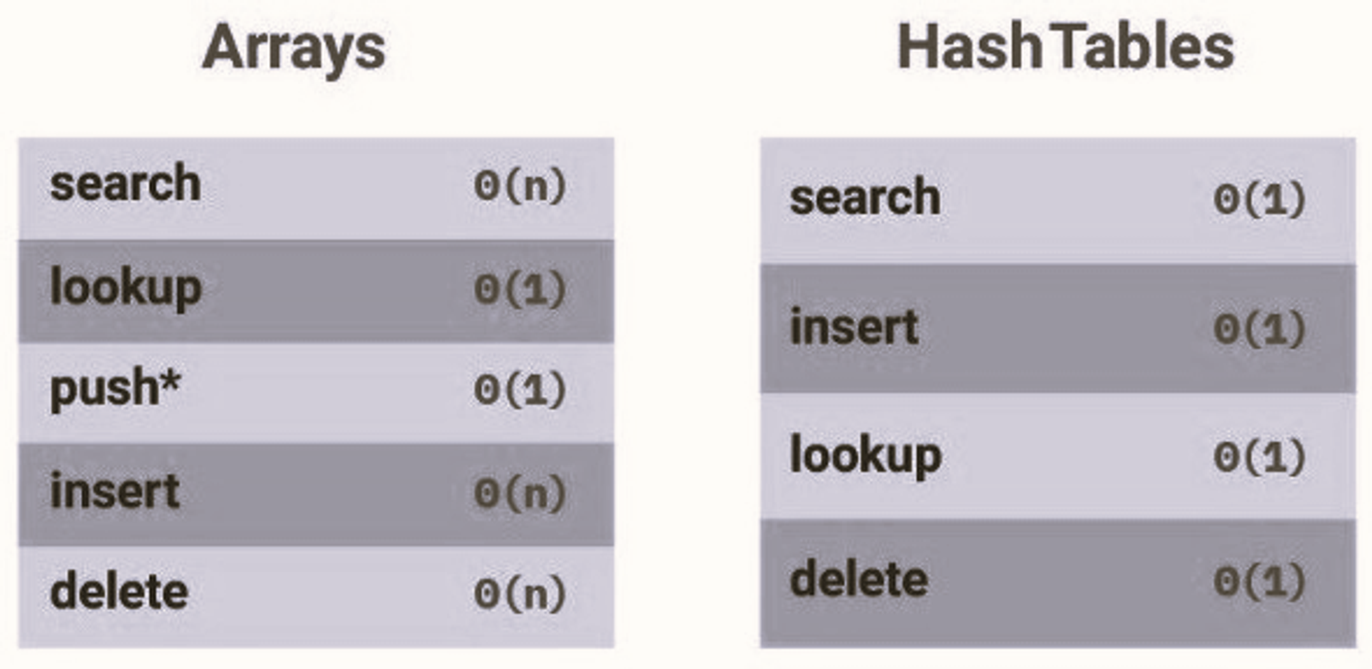
Hash Tables vs. Arrays
We've noticed a few differences between hash tables and arrays.
- When it comes to looking for items, hash tables are usually faster.
- In arrays, you must loop over all items before finding what you are looking for, while with a hash table, you go directly to the item's location.
- Inserting an item in Hash tables is also faster because you simply hash the key and insert it.
- In arrays shifting the items is important first before inserting another one.
Important Note: When choosing data structures for specific tasks, you must be extremely cautious, especially if they have the potential to harm the performance of your product.
Having an O(n) lookup complexity for functionality that must be real-time and relies on a large amount of data could make your product worthless.
Even if you feel that the correct decisions have been taken, it is always vital to verify that this is accurate and that your users have a positive experience with your product.
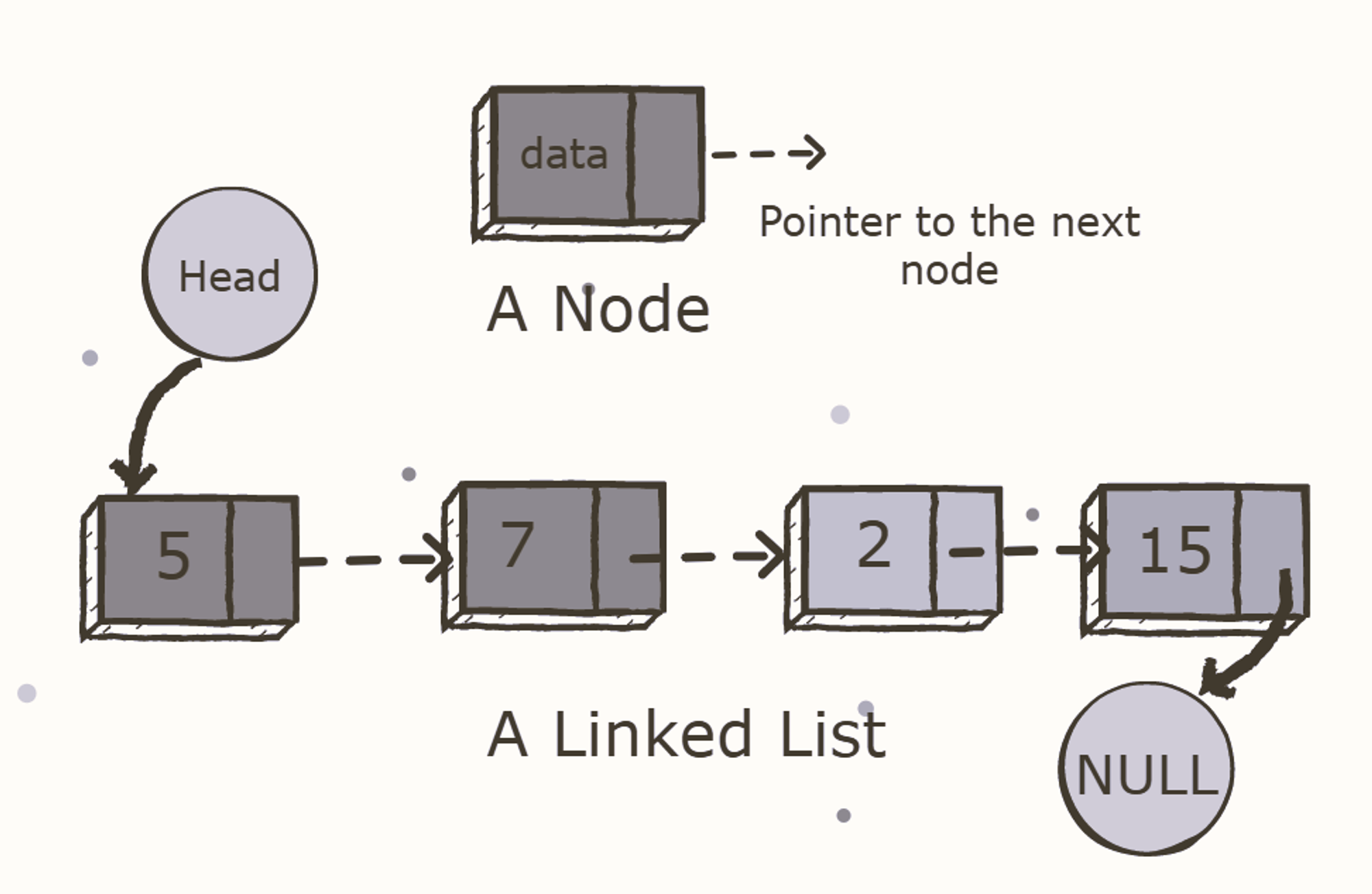
Linked Lists
A linked list is a common data structure made of one or more nodes. Each node contains a value and a pointer to the previous/next node forming the chain-like structure. These nodes are stored randomly in the system's memory, which improves its space complexity compared to the array.

What is a pointer?
In computer science, a pointer is an object in many programming languages that stores a memory address. This can be that of another value located in computer memory, or in some cases, that of memory-mapped computer hardware.
A pointer references a location in memory, and obtaining the value stored at that location is known as dereferencing the pointer.
As an analogy, a page number in a book's index could be considered a pointer to the corresponding page; dereferencing such a pointer would be done by flipping to the page with the given page number and reading the text found on that page.
EX:
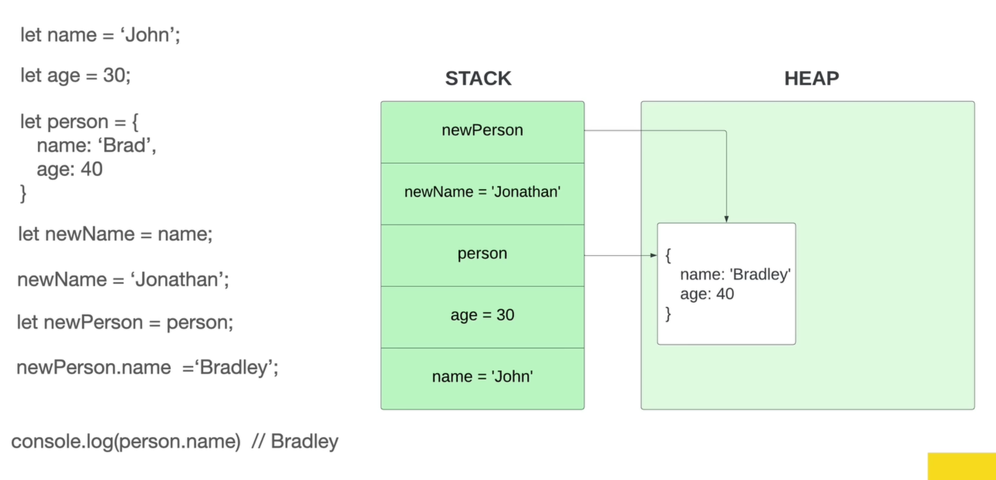
Person and newPerson in the example above both point to the same location in memory.
The BIG O of Linked-lists:
| prepend | O(1) |
|---|---|
| append | O(1) |
| lookup | O(n) |
| insert | O(n) |
| delete | O(n) |
Types of Linked Lists
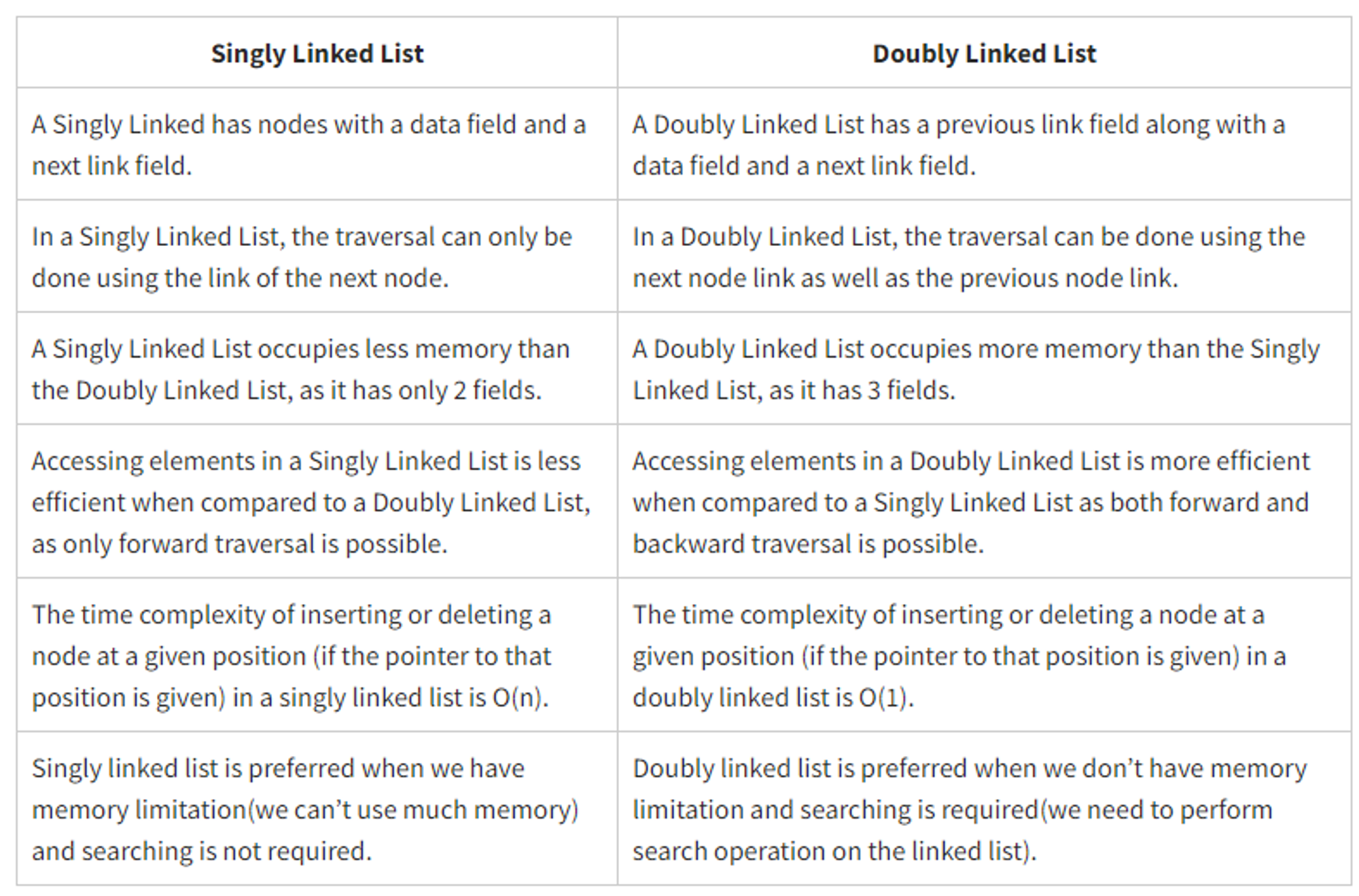
Singly linked list
The singly linked list (SLL) is a linear data structure comprising of nodes chained together in a single direction. Each node contains a data member holding useful information, and a pointer to the next node.
The problem with this structure is that it only allows us to traverse forward, i.e., we cannot iterate back to a previous node if required.
This is where the doubly linked list (DLL) shines. DLLs are an extension of basic linked lists with only one difference.
Doubly linked list
A doubly linked list contains a pointer to the next node as well as the previous node. This ensures that the list can be traversed in both directions.
From this definition, we can see that a DLL node has three fundamental members:
- the data
- a pointer to the next node
- a pointer to the previous node
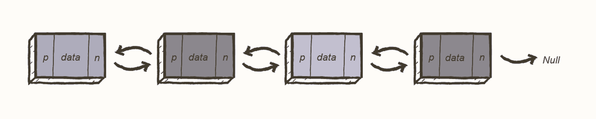
A DLL costs more in terms of memory due to the inclusion of a p (previous) pointer. However, the reward for this is that iteration becomes much more efficient.
Linked Lists Good at 😀:
- Fast insertion
- Fast deletion
- Ordered
- Flexible size
Linked Lists Bad at 😒:
- Slow Lookup
- More Memory
reverse() Logic
reverse() {
		if (!this.head.next){
			return this.head;
		}
		let prev = null;
		let next = null;
		this.tail = this.head;
		let current = this.head;
		while(current){
			next = current.next;
			current.next = prev;
			prev = current;
			current = next;
		}
		this.head = prev;
		return this;
	}
Stacks and Queues
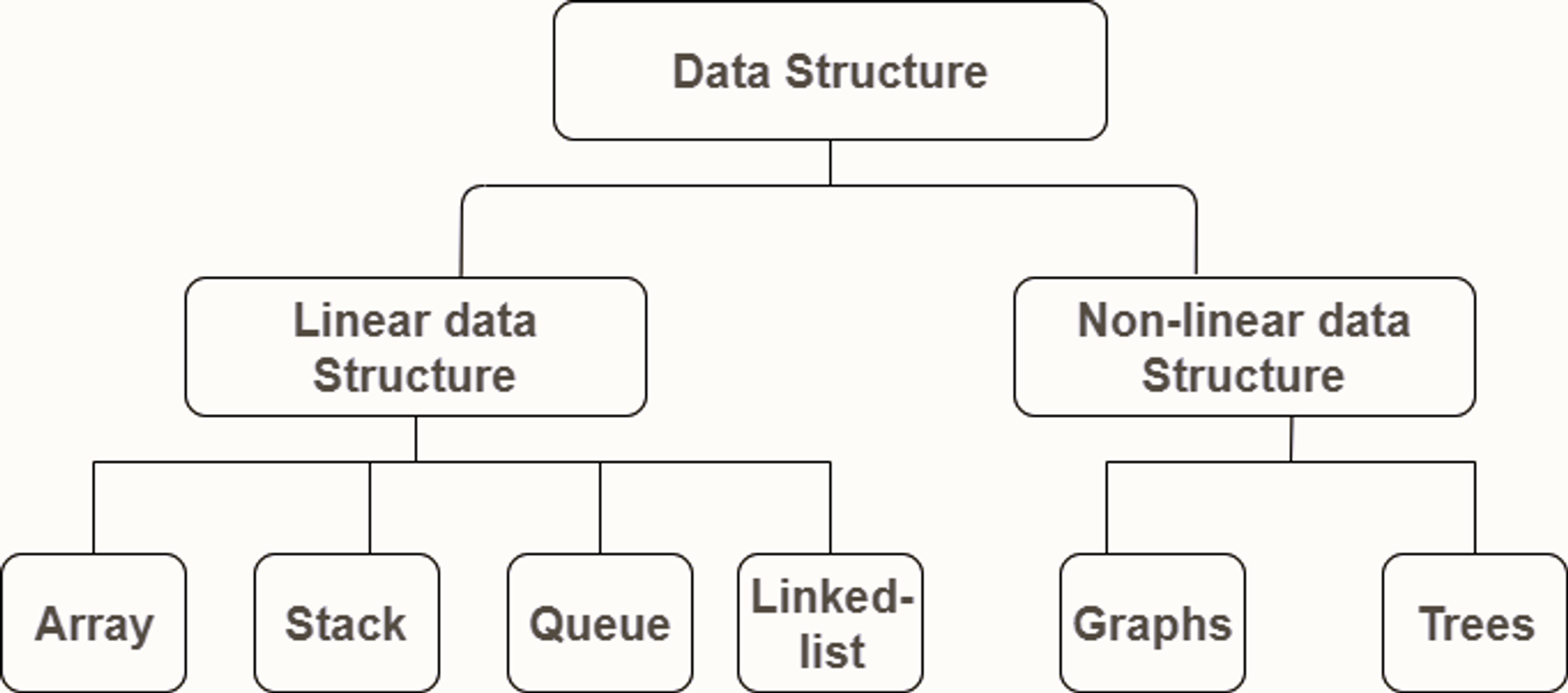
Stacks and Queues are both what we call linear data structures. Linear data structures allow us to traverse (that is go through) data elements sequentially (one by one) in which only one data element can be directly reached.
Now the reason that these are very similar is that they can be implemented in similar ways and the main difference is only how items get removed from this data structure.
Unlike an array in stacks and queues there's no random access operation. You mainly use stacks and queues to run commands like push, peak, pop. All of which deal exclusively with the element at the beginning or the end of the data structure.
Stacks
Stack is a linear data structure in which the element inserted last is the element to be deleted first.
It is also called Last In First Out (LIFO).
In a stack, the last inserted element is at the top.
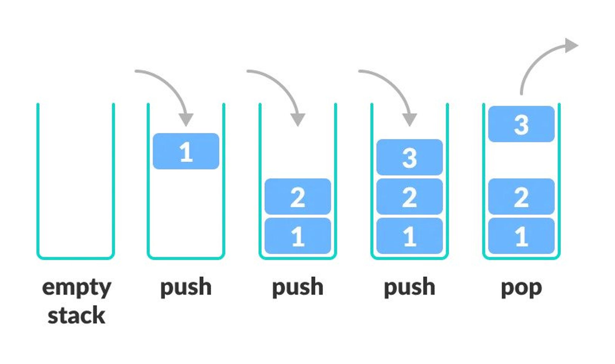
Operations
| push | Inserts an element into the stack at the end. | O(1) |
|---|---|---|
| peek | Returns the last inserted element. | O(n) |
| pop | Deletes and returns the last inserted element from the stack. | O(1) |
Queues
A queue is another common data structure that places elements in a sequence, similar to a stack. A queue uses the FIFO method (First In First Out), by which the first element that is enqueued will be the first one to be dequeued.
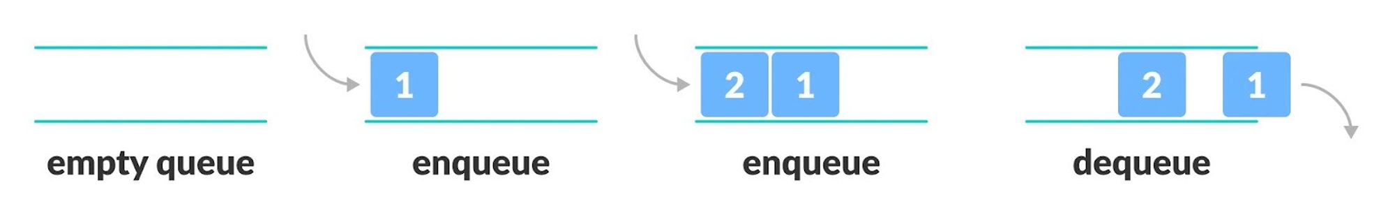
Operations
| enqueue | Inserts an element to the end of the queue | O(1) |
|---|---|---|
| dequeue | Removes an element from the start of the queue | O(1) |
| isempty | Returns true if the queue is empty. | O(1) |
| peek | Returns the first element of the queue | O(1) |
These higher-level data structures, which are built on top of lower-level ones like linked lists and arrays, are beneficial for limiting the operations you can perform on the lower-level ones.
In computer science, that is actually advantageous. The fact that you have this restricted control over a data structure is advantageous.
Users of this data structure solely carry out their efficient write operations. It's harder for someone to work if you give them all the tools in the world than if you simply give them two or three so they know exactly what they need to do.
Stacks and Queues Good at 😀:
- Fast Operations
- Fast Peek
- Ordered
Stacks and Queues Bad at 😒:
- Slow Lookup
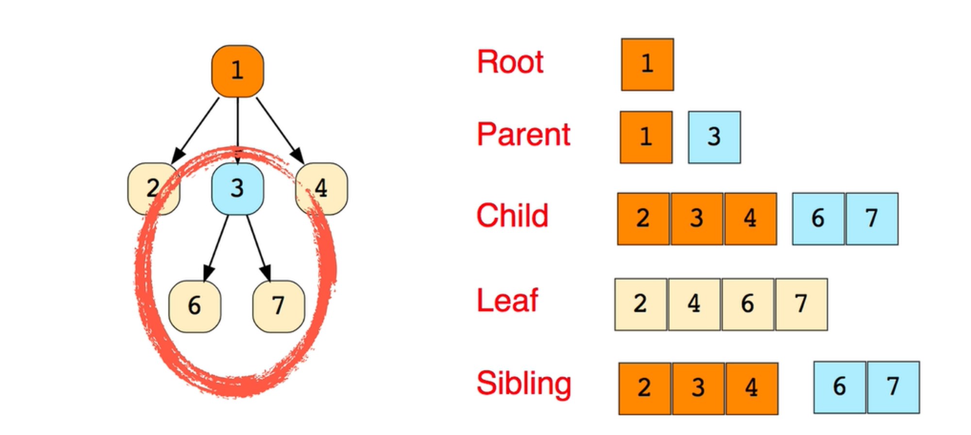
Trees
A Tree is a non-linear data structure and a hierarchy consisting of a collection of nodes such that each node of the tree stores a value and a list of references to other nodes (the “children”).
This data structure is a specialized method to organize and store data in the computer to be used more effectively.
It consists of a central node, structural nodes, and sub-nodes, which are connected via edges. We can also say that tree data structure has roots, branches, and leaves connected with one another.
Why is Tree considered a non-linear data structure?
The data in a tree are not stored in a sequential manner i.e, they are not stored linearly. Instead, they are arranged on multiple levels or we can say it is a hierarchical structure.
For this reason, the tree is considered to be a non-linear data structure.
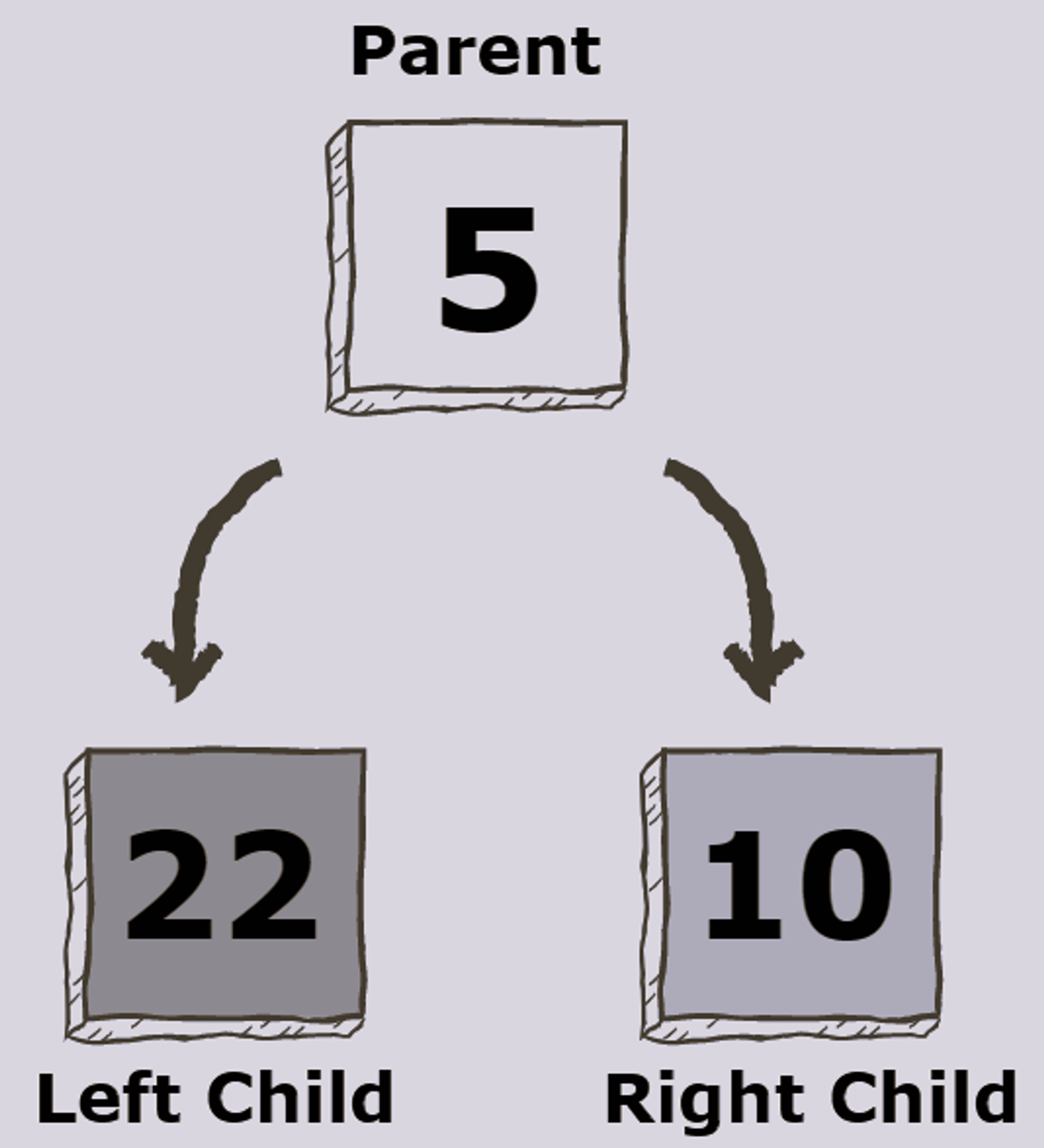
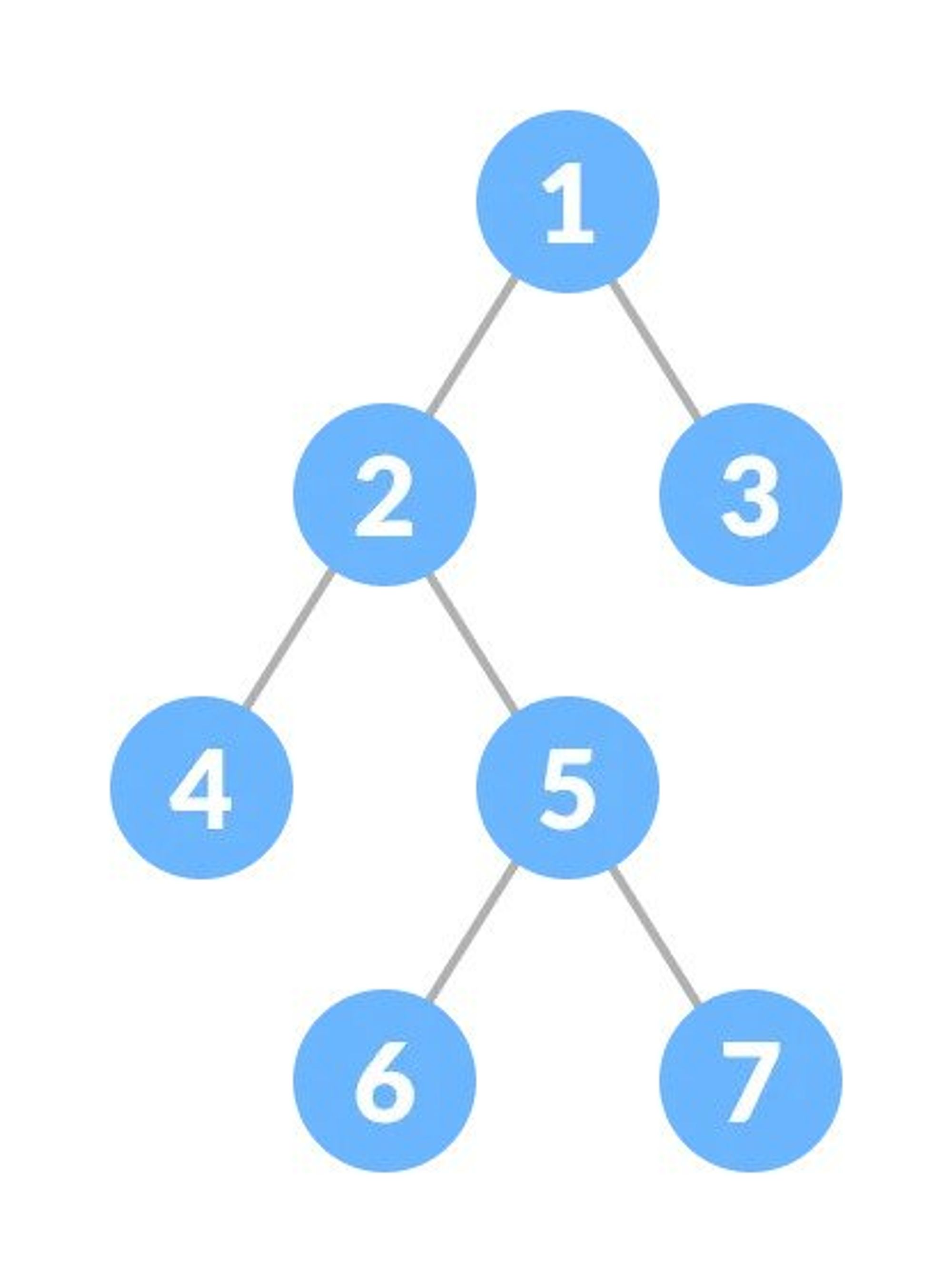
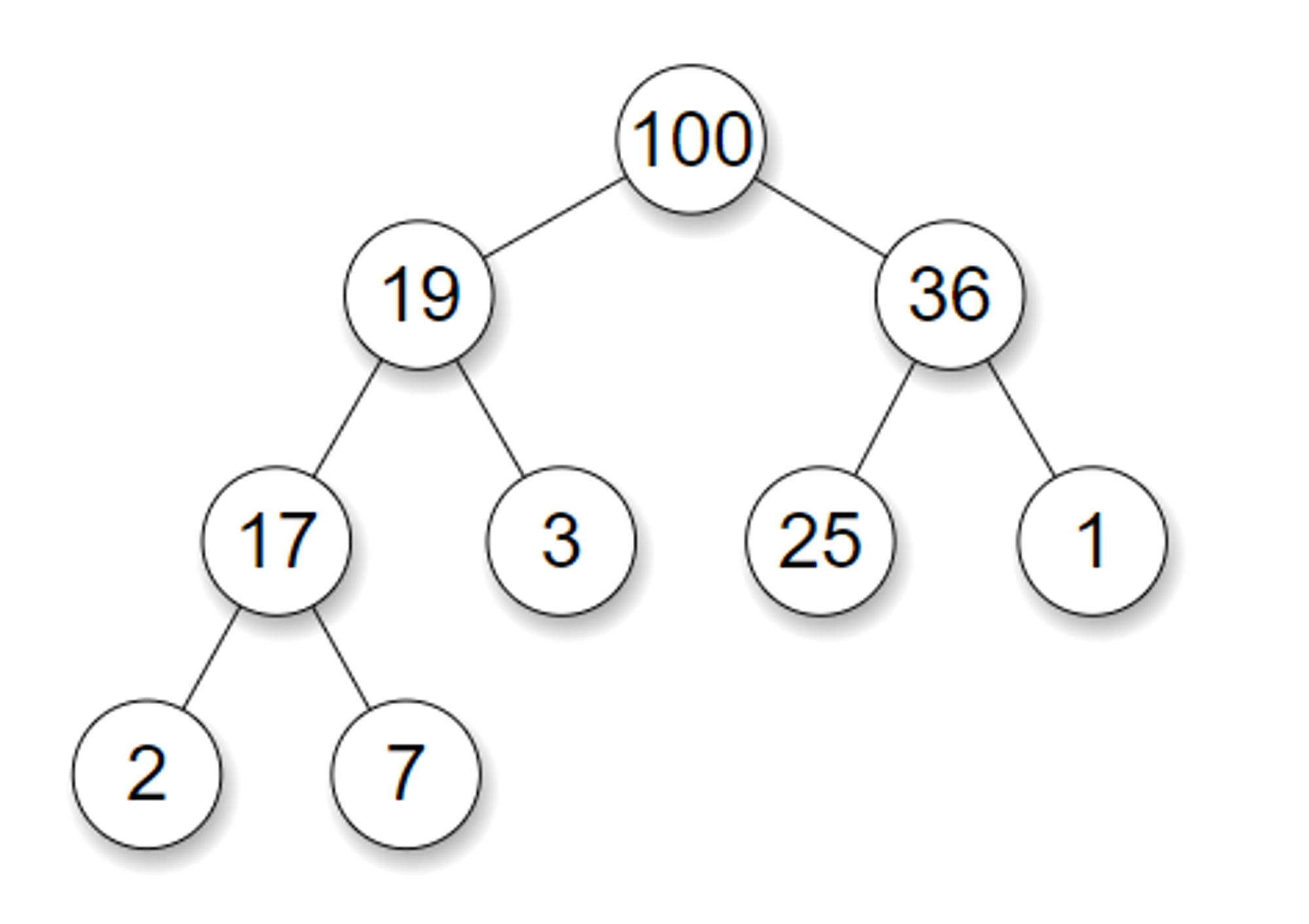
Binary Trees
A binary tree is a tree data structure composed of nodes, each of which has at most, two children, referred to as left and right nodes. The tree starts off with a single node known as the root.
Each node in the tree contains the following:
- Data
- Pointer to the left child
- Pointer to the right child
- In case of a leaf node, the pointers to the left and right child point to
null
Types Of Binary Trees
Full Binary Tree
A full Binary tree is a special type of binary tree in which every parent node/internal node has either two or no children.
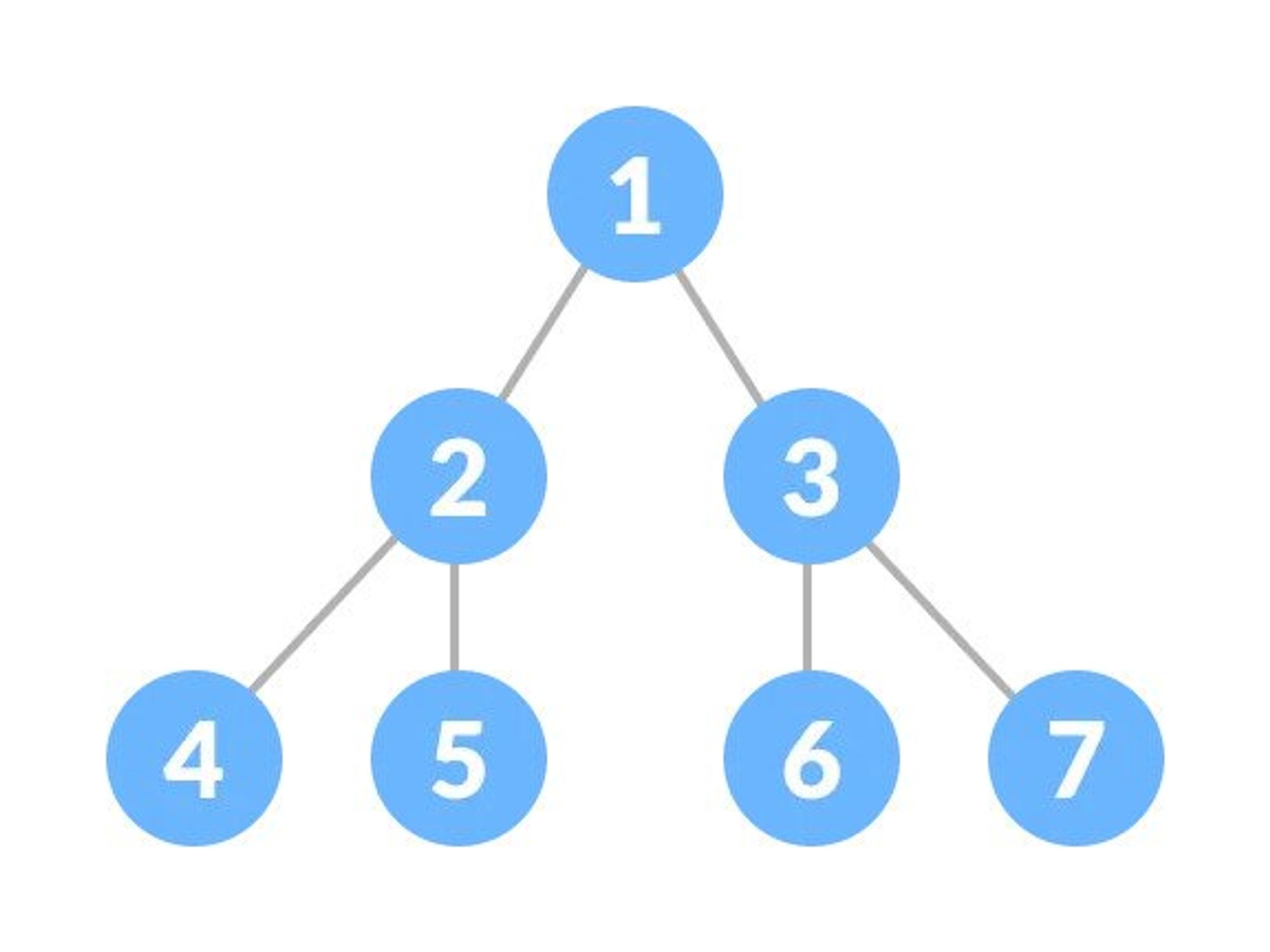
Perfect Binary Tree
A perfect binary tree is a type of binary tree in which every internal node has exactly two child nodes and all the leaf nodes are at the same level.
Complete Binary Tree
A complete binary tree is a binary tree in which all the levels are completely filled except possibly the lowest one, which is filled from the left.
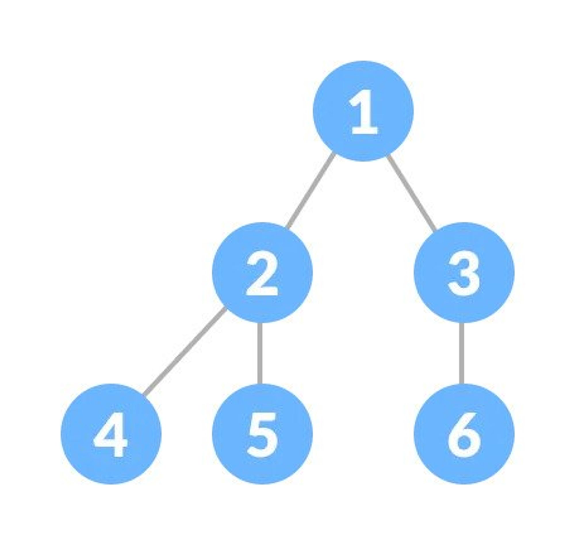
A complete binary tree is just like a full binary tree, but with two major differences:
- All the leaf elements must lean towards the left.
- The last leaf element might not have a right sibling i.e. a complete binary tree doesn't have to be a full binary tree.
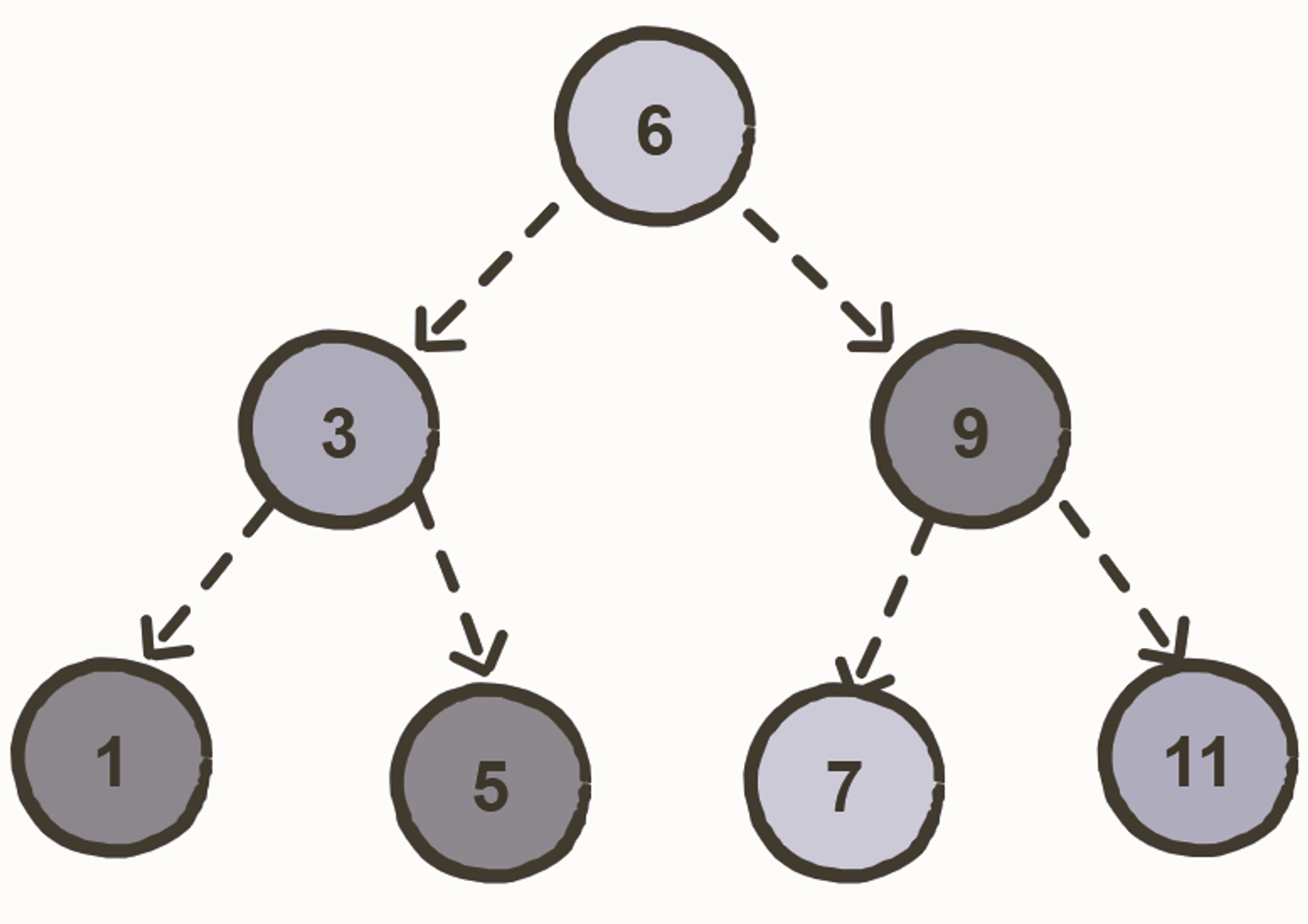
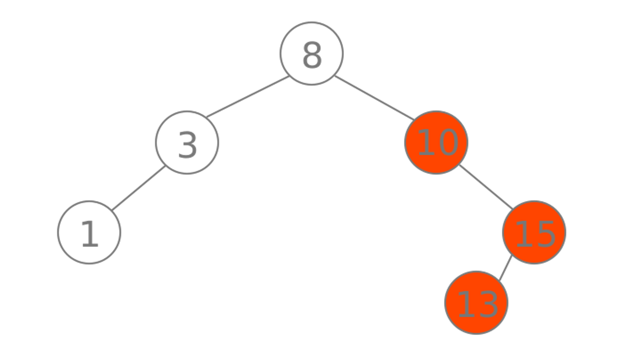
Binary Search Tree
A Binary Search Tree is a binary tree where each node contains a key and an optional associated value. It allows particularly fast lookup, addition, and removal of items.
The nodes are arranged in a binary search tree according to the following properties:
- The left subtree of a particular node will always contain nodes with keys less than that node’s key.
- The right subtree of a particular node will always contain nodes with keys greater than that node’s key.
- The left and the right subtree of a particular node will also, in turn, be binary search trees.
Time Complexity
In average cases, the above mentioned properties enable the insert, search and deletion operations in O(log n) time where n is the number of nodes in the tree.
However, the time complexity for these operations is O(n) in the worst case when the tree becomes unbalanced.
Space Complexity
The space complexity of a binary search tree is O(n) in both the average and the worst cases.
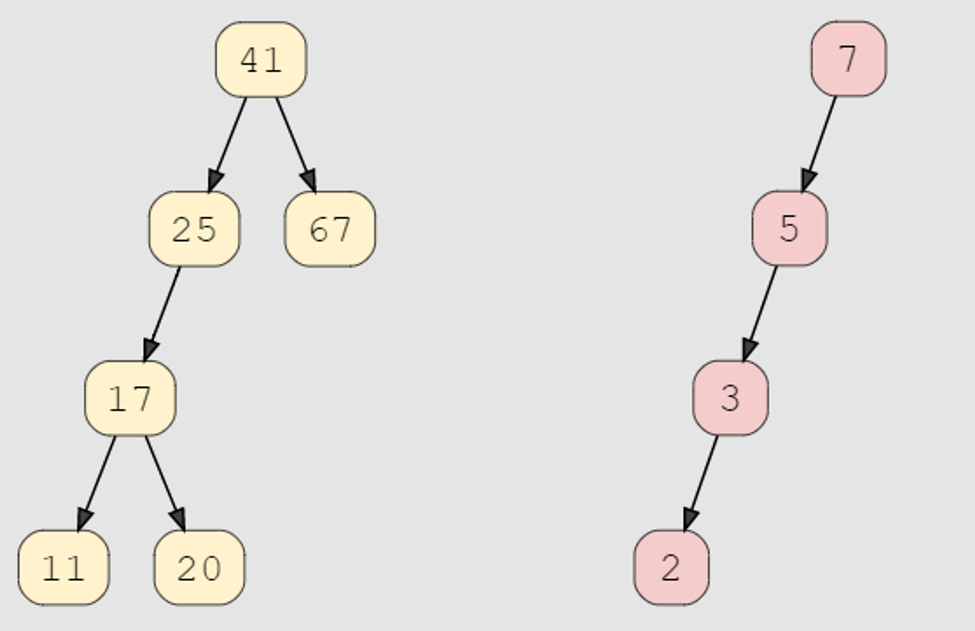
Balanced vs. Unbalanced BST
A binary tree is called balanced if every leaf node is not more than a certain distance away from the root than any other leaf.
That is, if we take any two leaf nodes (including empty nodes), the distance between each node and the root is approximately the same.
In most cases, "approximately the same" means that the difference between the two distances (root to first leaf and root to second leaf) is not greater than 1, but the exact number can vary from application to application.
This distance constraint ensures that it takes approximately the same amount of time to reach any leaf node in a binary tree from the root. A linked list is a kind of maximally-unbalanced binary tree.
Binary Search Tree Good at 😀:
- Better than O(n)
- Ordered
- Flexible Size
Binary Search Tree Bad at 😒:
- No O(1) operations
Balancing a Binary Search Tree
The primary issue with binary search trees is that they can be unbalanced. In the worst case, they are still not more efficient than a linked list, performing operations such as insertions, deletions, and searches in O(n) time.
AVL Trees
AVL trees are a modification of binary search trees that resolve this issue by maintaining the balance factor of each node.
Red-Black Trees
The red-black tree is another member of the binary search tree family. Like the AVL tree, a red-black tree has self-balancing properties.
Binary Heap
The binary heap is a binary tree (a tree in which each node has at most two children) which satisfies the following additional properties:
-
The binary tree is complete, i.e. every level except the bottom-most level is completely filled and nodes of the bottom-most level are positioned as left as possible.
-
A Binary Heap is either Min Heap or Max Heap. In a Min Binary Heap, the key at root must be minimum among all keys present in Binary Heap. The same property must be recursively true for all nodes in Binary Tree. Max Binary Heap is similar to MinHeap.
Notice that the binary tree does not enforce any ordering between the sibling nodes.
Also notice that the completeness of the tree ensures that the height of the tree is log(n), where n is the number of elements in the heap. The nodes in the binary heap are sorted with the priority queue method.
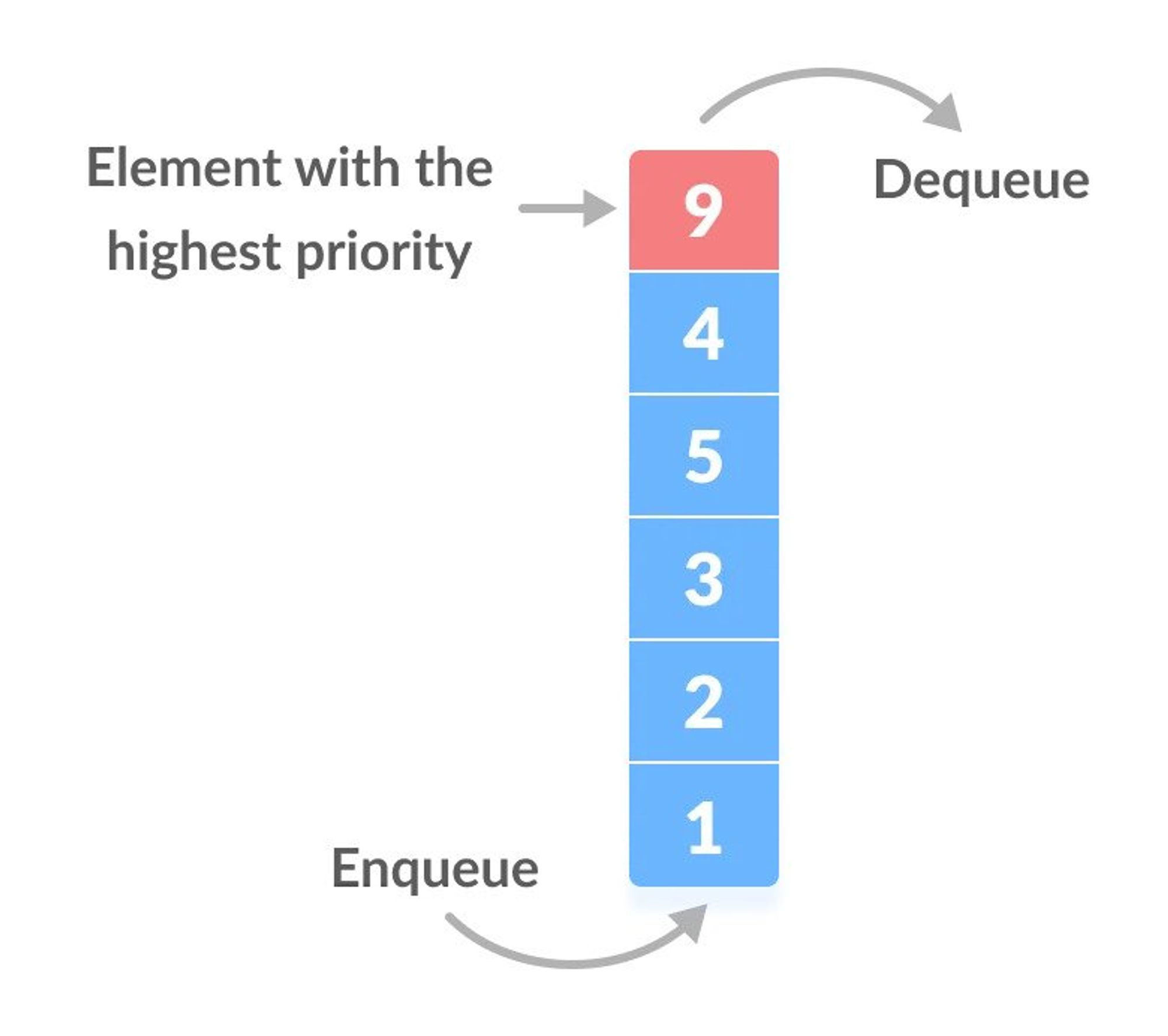
Priority Queue
A priority queue is a special type of queue in which each element is associated with a priority value. And, elements are served on the basis of their priority. That is, higher priority elements are served first.
However, if elements with the same priority occur, they are served according to their order in the queue.
Assigning Priority Value
Generally, the value of the element itself is considered for assigning the priority. For example, The element with the highest value is considered the highest priority element.
However, in other cases, we can assume the element with the lowest value as the highest priority element. We can also set priorities according to our needs.
Priority Queue vs. Normal Queue
In a queue, the first-in-first-out rule is implemented whereas, in a priority queue, the values are removed on the basis of priority. The element with the highest priority is removed first.
Binary Heap Good at 😀:
- Better than O(n)
- Priority
- Flexible Size
- Fast Insert
Binary Heap Bad at 😒:
- Slow Lookup
Trie or Prefix Tree or Radix Tree or Digital Tree
A trie is a special tree that can compactly store strings. Here's a trie that stores ‘this’, ‘there’, ‘that’, ‘does’, ‘did’.
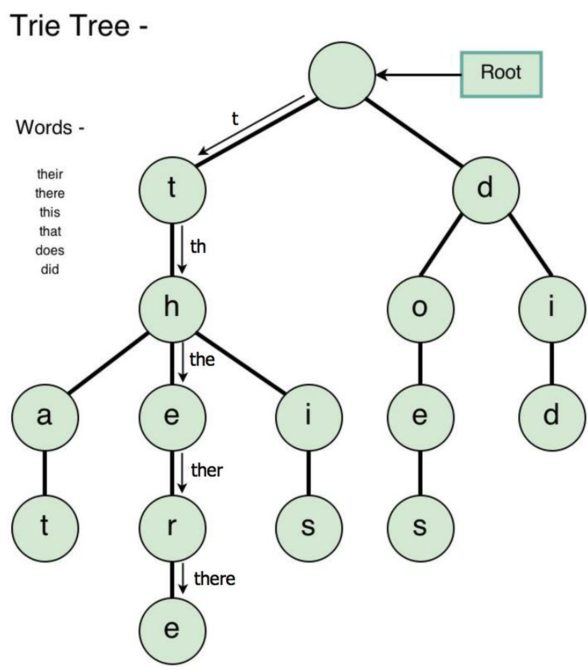
Notice that we only store "there" once, even though it appears in two strings: "that" and "this".
Trie Strengths 😀:
- Sometimes Space-Efficient. If you're storing lots of words that start with similar patterns, tries may reduce the overall storage cost by storing shared prefixes once.
- Efficient Prefix Queries. Tries can quickly answer queries about words with shared prefixes, like:
- How many words start with "choco"?
- What's the most likely next letter in a word that starts with "strawber"?
Trie Weaknesses 😒:
- Usually Space-Inefficient. Tries rarely save space when compared to storing strings in a set.
- ASCII characters in a string are one byte each. Each link between trie nodes is a pointer to an address—eight bytes on a 64-bit system. So, the overhead of linking nodes together often outweighs the savings from storing fewer characters.
- Not Standard. Most languages don't come with a built-in trie implementation. You'll need to implement one yourself.
Tries Time Complexity: O (length of the word)
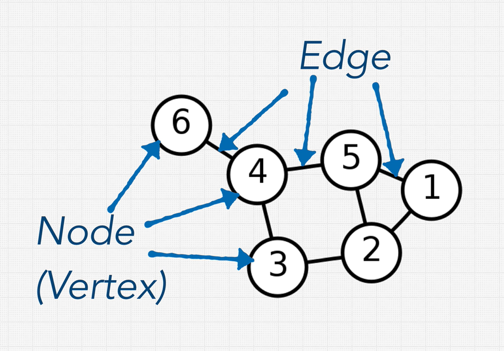
Graphs
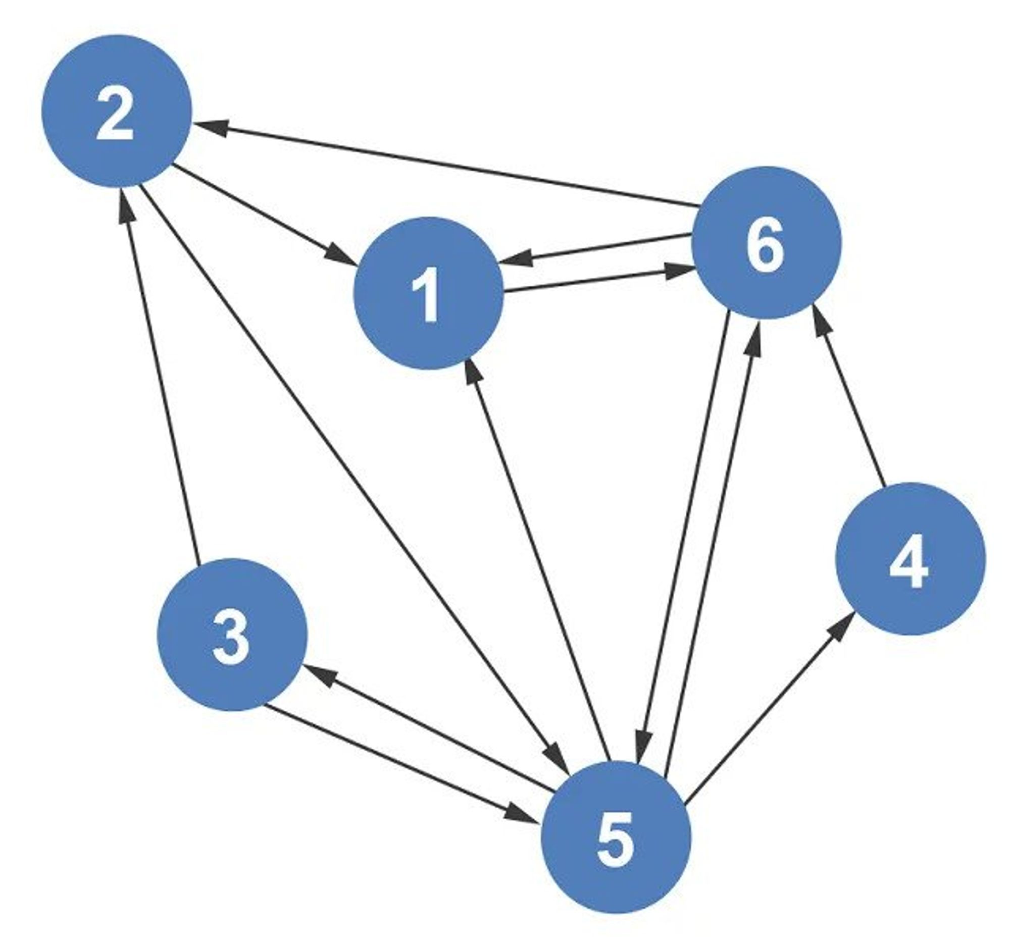
The Graph data structure is a collection of nodes. But unlike with trees, there are no rules about how nodes should be connected. There are no root, parent, or child nodes. Also, nodes are called vertices and they are connected by edges.
Usually, graphs have more edges than vertices. Graphs with more edges than vertices are called dense graphs. If there are fewer edges than vertices, then it’s a sparse graph.
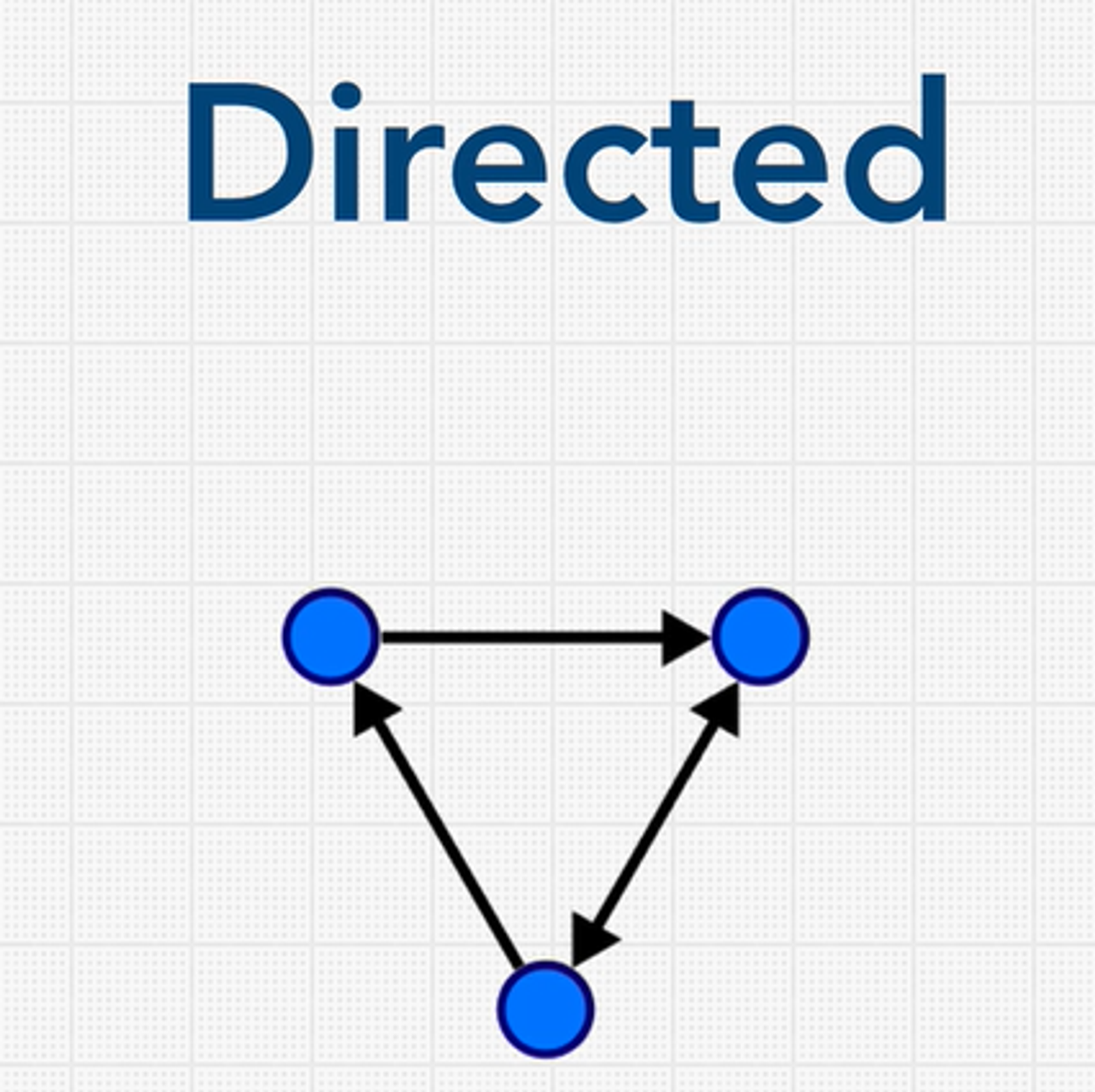
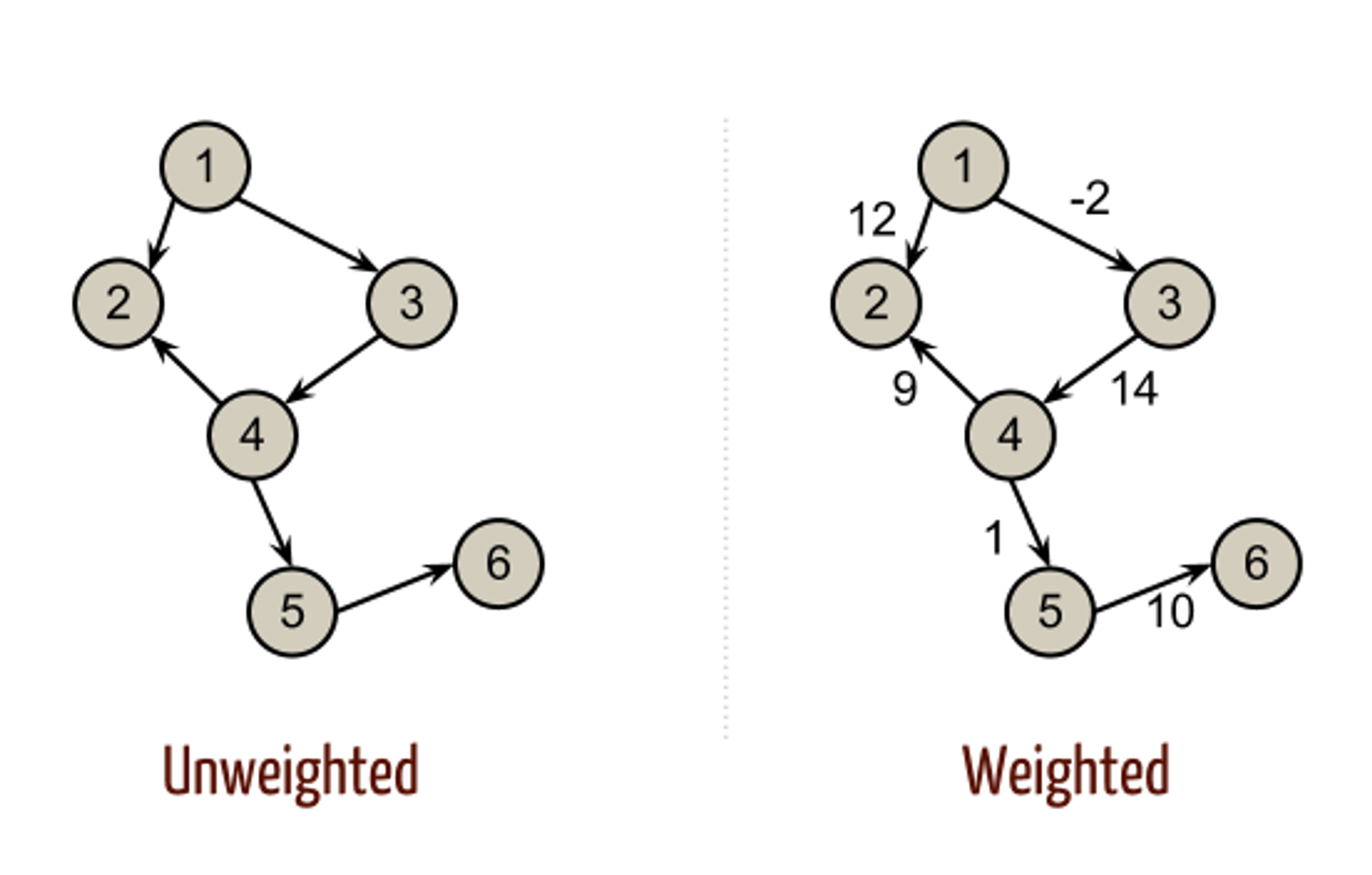
In some graphs, the edges are directional. These are known as directed graphs or digraphs.
Graphs are considered to be connected if there is a path from each vertex to another.
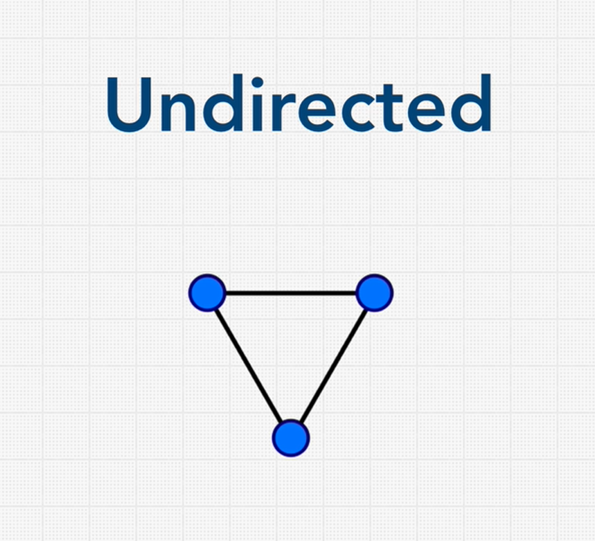
Graphs whose edges are all bidirectional are called undirected graphs, unordered graphs, or just graphs. These types of graphs have no implied direction on edges between the nodes. Edge can be traversed in either direction.
By default, graphs are assumed to be unordered.
In some graphs, edges can have a weight. These are called weighted graphs. So, when I say edges have a weight, what I mean to say is that they have some numbers which typically shows the cost of traversing in a graph.
When we are concerned with the minimum cost of traversing the graph then what we do is we find the path that has the least sum of those weights.
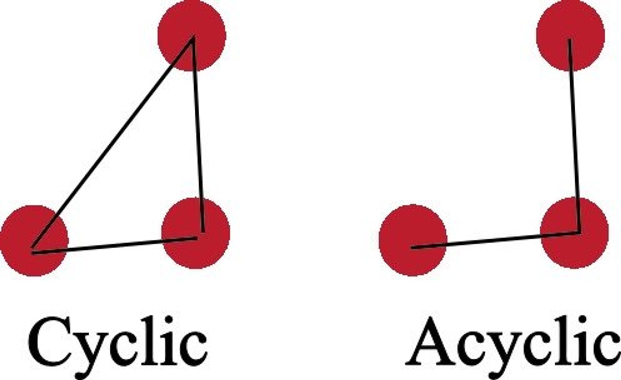
Cyclic graphs are a sort of graph in which the starting vertex also serves as the final vertex. Trees are a special type of graph that includes a path from the starting vertex (the root) to some other vertex. Therefore, trees are Acyclic Graphs.
Representing Graphs
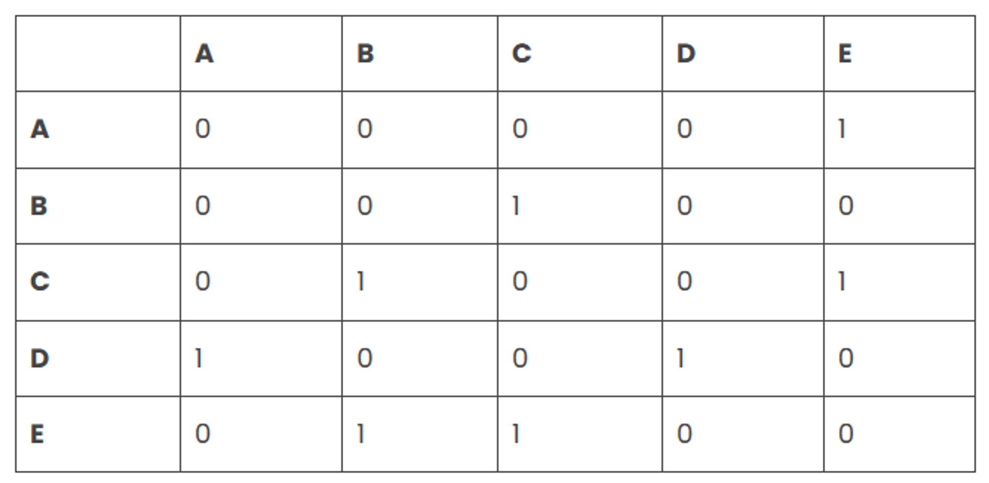
A graph can be represented using 3 data structures- adjacency matrix, adjacency list and Edge List.
An adjacency matrix can be thought of as a table with rows and columns. The row labels and column labels represent the nodes of a graph. An adjacency matrix is a square matrix where the number of rows, columns and nodes are the same. Each cell of the matrix represents an edge or the relationship between two given nodes.
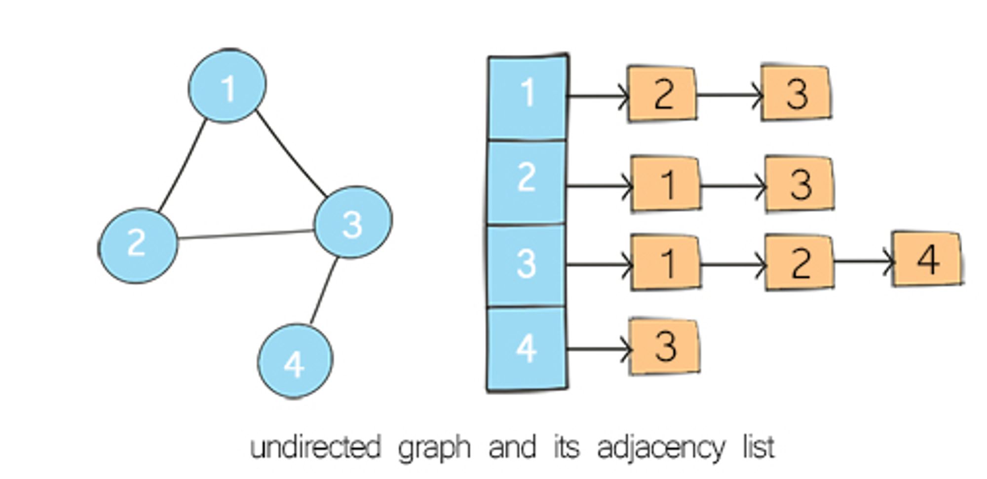
In adjacency list representation of a graph, every vertex is represented as a node object. The node may either contain data or a reference to a linked list. This linked list provides a list of all nodes that are adjacent to the current node
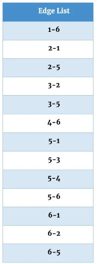
The Edge List is another way to represent adjacent vertices. It is much more efficient when trying to figure out the adjacent nodes in a graph. The edge list contains a list of edges in alphanumerical order.
Graphs Good at 😀:
- Relationships
Graphs Bad at 😒:
- Scaling is hard
Algorithms Cheat Sheet
What is an Algorithm?
An algorithm is a set of instructions or a step-by-step procedure used to solve a problem or perform a specific task.
In computer science, algorithms are typically used to solve computational problems, such as sorting a list of numbers, searching for a particular item in a database, or calculating the shortest path between two points on a graph.
When do I need to use Algorithms?
They are used whenever you need to perform a specific task that can be broken down into smaller, well-defined steps.
Some examples of situations where you might use algorithms include:
- Sorting data
- Searching for information
- Calculating mathematical functions
- Optimizing performance
- Machine learning
Algorithms are typically evaluated based on their efficiency, expressed in terms of time complexity and space complexity.
Time complexity refers to the amount of time required for the algorithm to produce the output.
Space complexity refers to the amount of memory or storage required by the algorithm.
Efficient algorithms are important because they allow us to solve problems quickly and with fewer resources.
In some cases, the difference between an efficient algorithm and an inefficient algorithm can be the difference between a problem being solvable and unsolvable.
Overall, algorithms are a fundamental concept in computer science and are used extensively in software development, data analysis, and many other fields.
Recursion
Recursion is a fundamental concept in programming when learning about data structures and algorithms. So, what exactly is recursion?
The process in which a function calls itself directly or indirectly is called recursion and the corresponding function is called a recursive function.
Recursive algorithm is essential to divide and conquer paradigm, whereby the idea is to divide bigger problems into smaller subproblems and the subproblem is some constant fraction of the original problem.
The way recursion works is by solving the smaller subproblems individually and then aggregating the results to return the final solution.
Stack Overflow
So what happens if you keep calling functions that are nested inside each other? When this happens, it’s called a stack overflow. And that is one of the challenges you need to overcome when it comes to recursion and recursive algorithms.
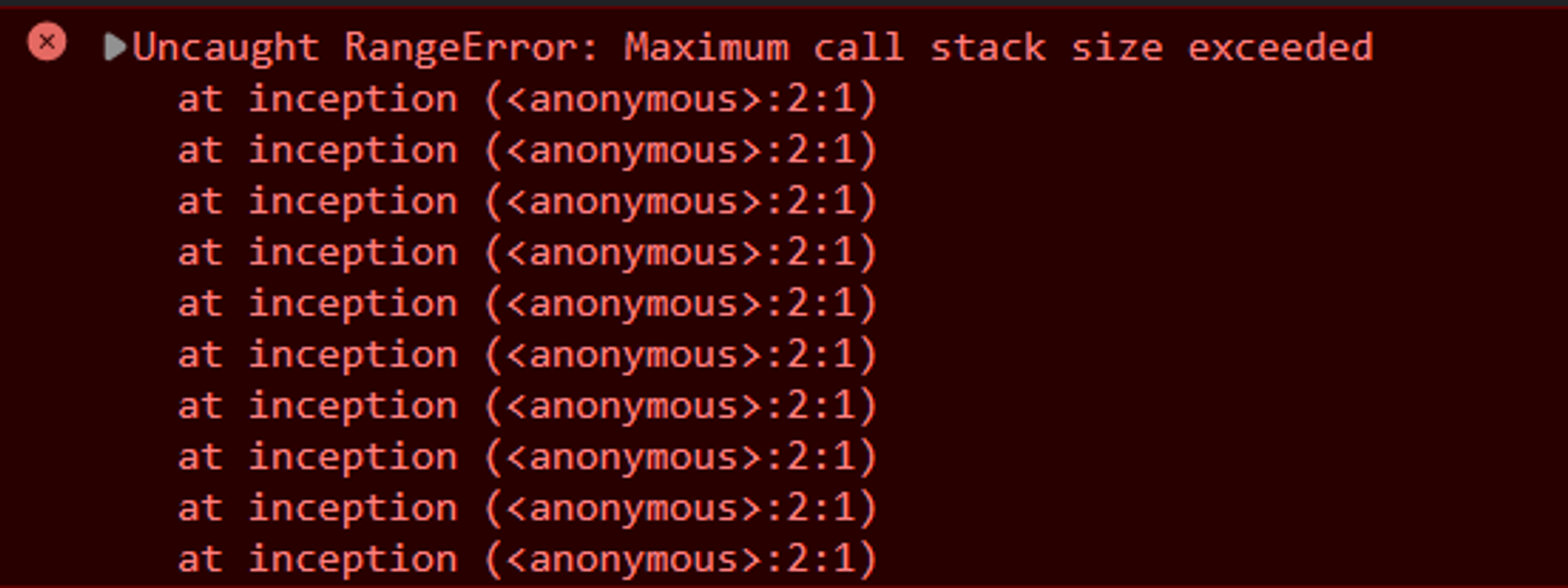
// When a function calls itself,
// it is called RECURSION
function inception() {
inception();
}
inception();
// returns Uncaught RangeError:
// Maximum call stack size exceeded
Avoiding Stack Overflow
In order to prevent stack overflow bugs, you must have a base case where the function stops making new recursive calls.
If there is no base case then the function calls will never stop and eventually a stack overflow will occur.
Here is an example of a recursive function with a base case. The base case is when the counter becomes bigger than 3.
let counter = 0;
function inception() {
    console.log(counter)
    if (counter > 3) {
        return 'done!';
    }
    counter++
    return inception();
}
When you run this program, the output will look like this:
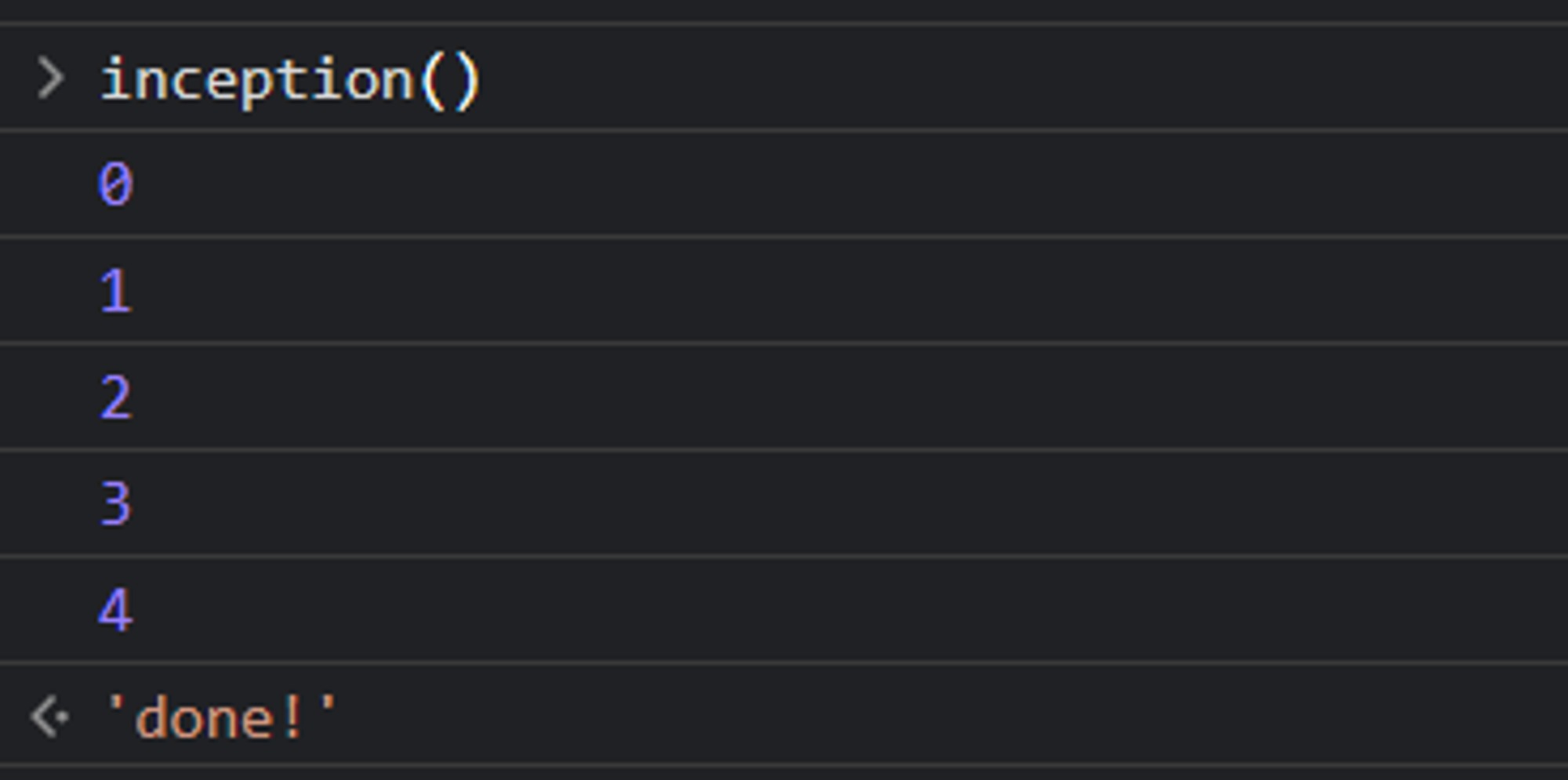
This program does not have a stack overflow error because once the counter is set to 4, the if statement’s condition will be True and the function will return ‘done!’, and then the rest of the calls will also return ‘done!’ in turn.
Example 1: Factorial
// Write two functions that find the factorial of any
// number. One should use recursive, the other should just
// use a for loop

function findFactoriatIterative(num){ // O(n)
    let res = num;
    for (let i = num; i > 0; i--){
        if (i != 1){
        res = res * (i-1);
        }
    }
    // console.log(res)
    return res

}

function findFactoriatRecursive(num){ // O(n)
    if (num == 2) {
        return 2;
    }
    return num * findFactoriatRecursive(num-1)
}

findFactoriatIterative(5)

// Output: 120
Example 2: Fibonacci
// Given a number N return the index value of the Fibonacci
// sequence, where the sequence is:

// o, 1, 1, 2, 3, 5, 8, 13, 21, 34, 55, 89, 144 ...
// the pattern of the sequence is that each value is the sum of
// the 2 previous values, that means that for N=5 -> 2+3

function fibonacciIterative(n){
    let arr = [0,1];
    for (let i = 2; i < n +1; i++){ // O(n)
        arr.push(arr[i-2] + arr[i-1]);
    }
    console.log(arr[n])
    return arr[n]
}

// fibonacciIterative(3);

function fibonacciRecursive(n) { // O(2^n)
    if (n < 2) {
        return n;
    }
    return fibonacciRecursive(n-1) + fibonacciRecursive(n-2)
}

fibonacciRecursive(3);

// Output: 2
Recursion vs. Iteration
| Recursion | Iteration |
|---|---|
| Recursion uses the selection structure. | Iteration uses the repetition structure. |
| Infinite recursion occurs if the step in recursion doesn't reduce the problem to a smaller problem. It also becomes infinite recursion if it doesn't convert on a specific condition. This specific condition is known as the base case. | An infinite loop occurs when the condition in the loop doesn't become False ever. |
| The system crashes when infinite recursion is encountered. | Iteration uses the CPU cycles again and again when an infinite loop occurs. |
| Recursion terminates when the base case is met. | Iteration terminates when the condition in the loop fails. |
| Recursion is slower than iteration since it has the overhead of maintaining and updating the stack. | Iteration is quick in comparison to recursion. It doesn't utilize the stack. |
| Recursion uses more memory in comparison to iteration. | Iteration uses less memory in comparison to recursion. |
| Recursion reduces the size of the code. | Iteration increases the size of the code. |
Recursion Good at 😀:
- DRY
- Readability
Recursion Bad at 😒:
- Large Stack
When do I need to use Recursion?
Every time you are using a tree or converting Something into a tree, consider Recursion.
1 . Divided into a number of subproblems that are smaller instances of the same problem.
-
Each instance of the subproblem is identical in nature.
-
The solutions of each subproblem can be combined to solve the problem at hand.
Sorting Algorithms
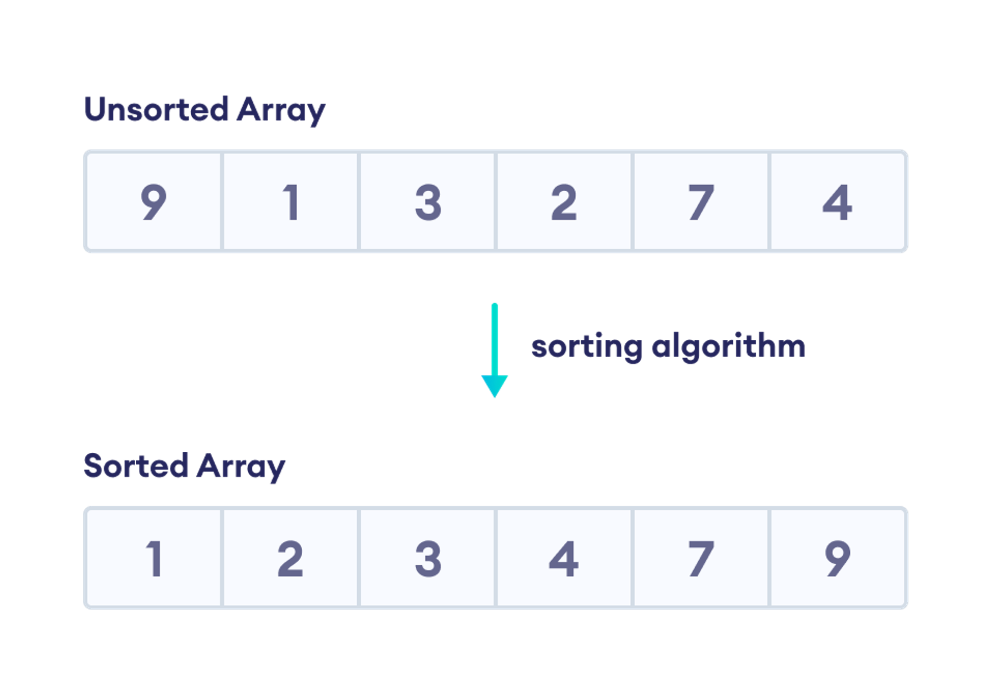
A sorting algorithm is used to arrange elements of an array/list in a specific order.
Sorts are most commonly in numerical or a form of alphabetical (or lexicographical) order, and can be in ascending (A-Z, 0-9) or descending (Z-A, 9-0) order.
What's all the fuss with sorting?
- Sorting algorithms are important because they make it easier and faster to access and process data
- They are a fundamental part of computer science and good programming practice
- They can be used to optimize many different operations
- They have numerous real-world applications in fields such as database management and finance.
Overall, understanding and using sorting algorithms effectively can help improve the performance and efficiency of software systems and data processing operations.
Why then can't we just use the sort() method that is already built in?
While the sort() method is a convenient built-in method provided by many programming languages to sort elements, it may not always be the best solution.
- The performance of sort() can vary depending on the size and type of data being sorted
- It may not maintain the order of equal elements
- It may not provide the flexibility to customize sorting criteria
- It may require additional memory to sort large datasets.
Therefore, in some cases, other sorting algorithms or custom sorting functions may be more efficient or appropriate.
Why are there so many different sorting algorithms?
There are many different sorting algorithms because each algorithm has its own strengths and weaknesses, and may be more appropriate for certain types of data or situations.
Factors that can influence the choice of sorting algorithm include performance, stability, in-place sorting, data distribution, and implementation complexity.
Therefore, there are many different sorting algorithms to choose from, each with its own unique characteristics, to provide a variety of options for different use cases.
Bubble Sort
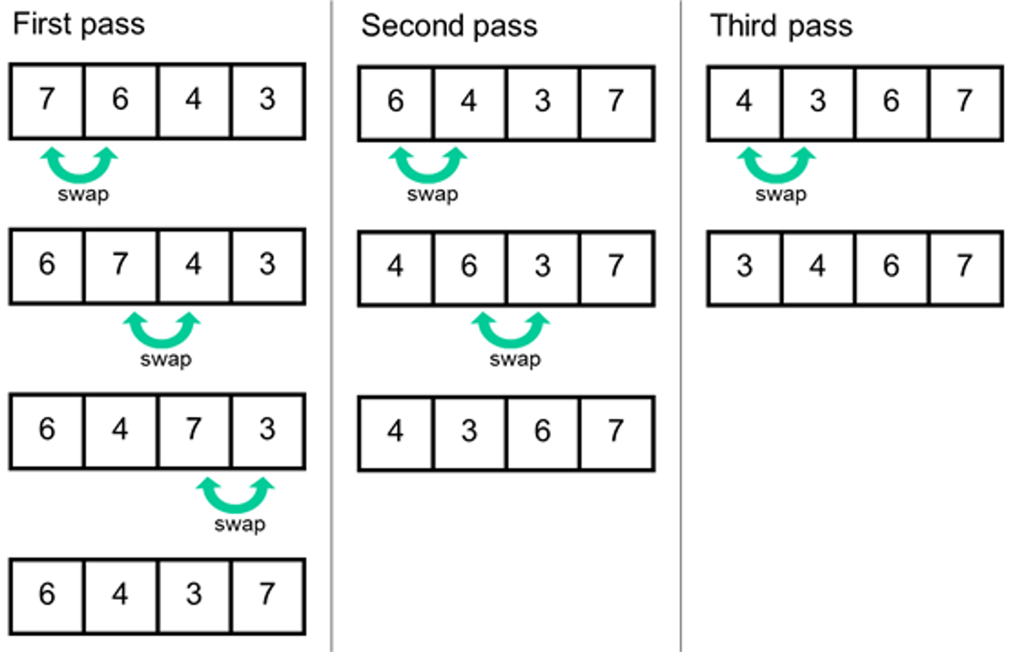
Bubble Sort is a simple sorting algorithm that repeatedly steps through a list of elements, compares adjacent elements and swaps them if they are in the wrong order.
The algorithm gets its name from the way smaller elements "bubble" to the top of the list with each iteration.
Here are the basic steps of the Bubble Sort algorithm:
- Starting at the beginning of the list, compare each pair of adjacent elements.
- If the elements are in the wrong order (e.g., the second element is smaller than the first), swap them.
- Continue iterating through the list until no more swaps are needed (i.e., the list is sorted).
The list is now sorted. Bubble Sort has a time complexity of O(n^2), making it relatively slow for large datasets.
However, it is easy to understand and implement, and can be useful for small datasets or as a starting point for more optimized sorting algorithms.
Implementation in JavaScript
const numbers = [99, 44, 6, 2, 1, 5, 63, 87, 283, 4, 0];

function bubbleSort(array) {
    for (let i =0; i < array.length; i++){
        for (let j =0; j < array.length; j++){
            if (array[j] > array[j+1]){
                let temp = array[j];
                array[j] = array[j+1];
                array[j + 1] = temp;
            }
        }
    }
}

bubbleSort(numbers)
console.log(numbers)
Output
PS D:\Coding Playground> node playground2.js
[
    0,  1,  2,  4,  5, 6, 44, 63, 87, 99, 283
]
Selection Sort
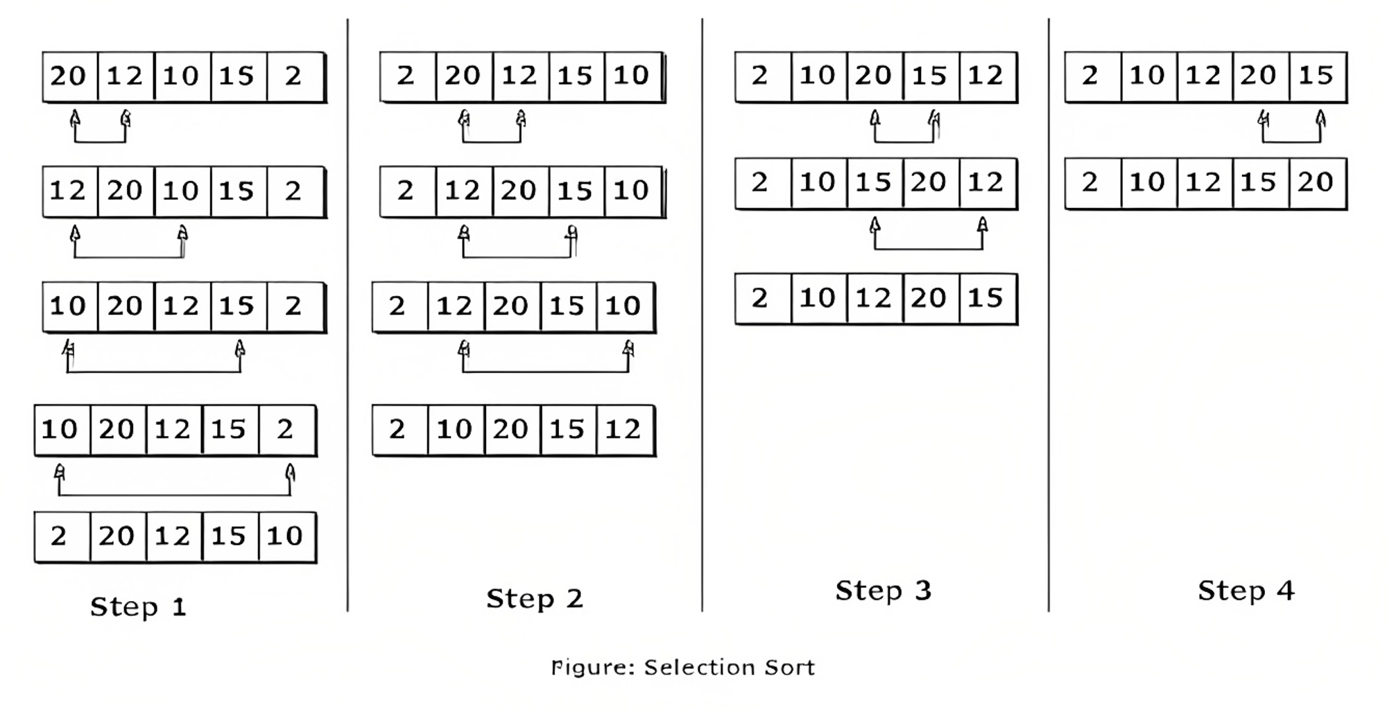
Selection Sort is another simple sorting algorithm that repeatedly finds the smallest element in an unsorted portion of an array and moves it to the beginning of the sorted portion of the array.
Here are the basic steps of the Selection Sort algorithm:
- Starting with the first element in the array, search for the smallest element in the unsorted portion of the array.
- Swap the smallest element found in step 1 with the first element in the unsorted portion of the array, effectively moving the smallest element to the beginning of the sorted portion of the array.
- Repeat steps 1 and 2 for the remaining unsorted elements in the array until the entire array is sorted.
The array is now sorted. Selection Sort has a time complexity of O(n^2), making it relatively slow for large datasets.
However, it is easy to understand and implement, and can be useful for small datasets or as a starting point for more optimized sorting algorithms.
Implementation in JavaScript
const numbers = [99, 44, 6, 2, 1, 5, 63, 87, 283, 4, 0];

function selectionSort(array) {
    const length = array.length;
    for(let i = 0; i < length; i++){
      // set current index as minimum
      let min = i;
      let temp = array[i];
      for(let j = i+1; j < length; j++){
        if (array[j] < array[min]){
          // update minimum if current is lower that what we had previously
          min = j;
        }
      }
      array[i] = array[min];
      array[min] = temp;
    }
    return array;
  }

selectionSort(numbers);
console.log(numbers);
Output
PS D:\Coding Playground> node playground2.js
[
    0,  1,  2,  4,  5, 6, 44, 63, 87, 99, 283
]
Insertion Sort
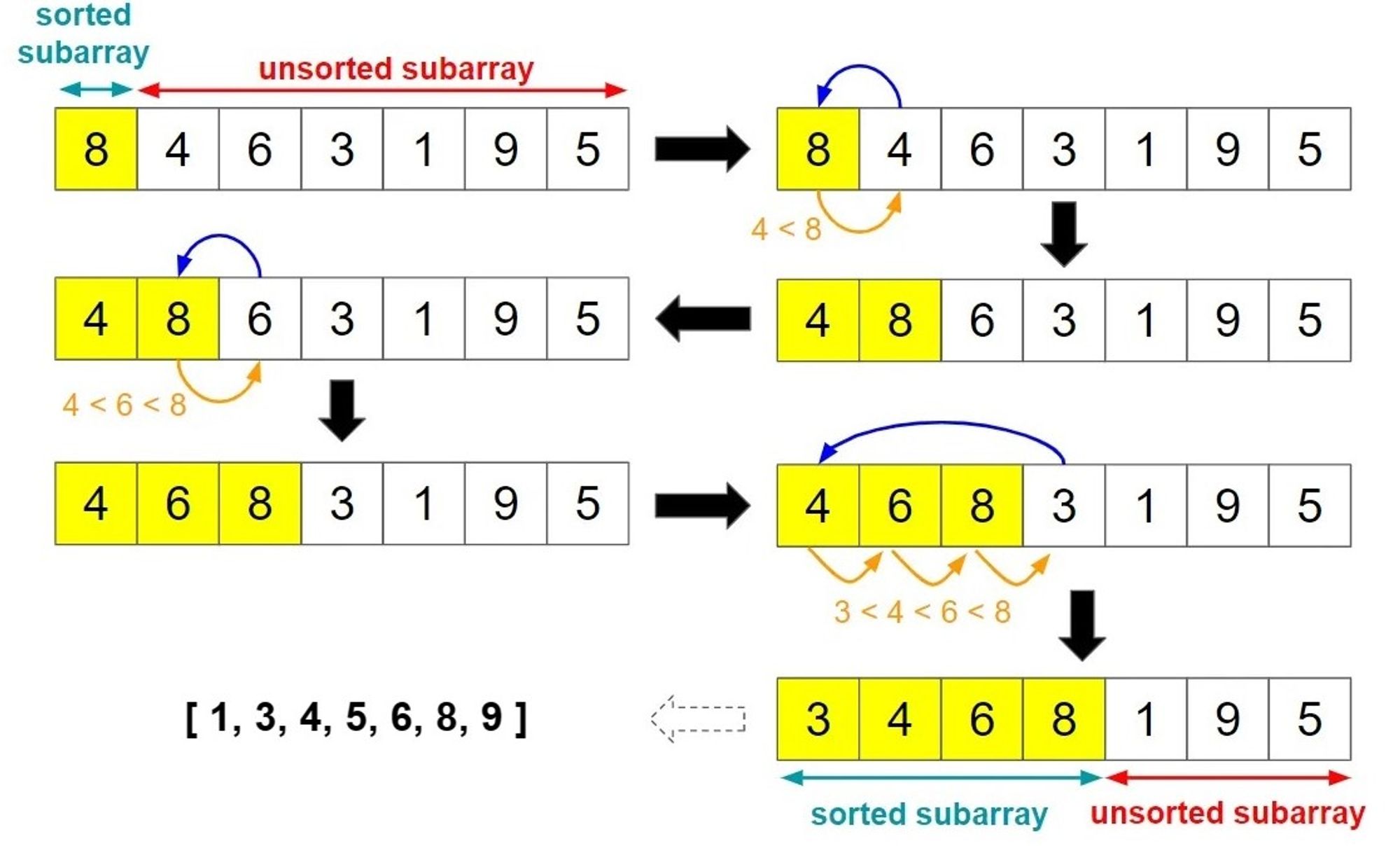
Insertion Sort is also another simple sorting algorithm that works by iteratively inserting each element of an array into its correct position within a sorted subarray.
Here are the basic steps of the Insertion Sort algorithm:
- Starting with the second element in the array, iterate through the unsorted portion of the array.
- For each element, compare it to the elements in the sorted portion of the array and insert it into the correct position.
- Repeat step 2 for all remaining elements in the unsorted portion of the array until the entire array is sorted.
Insertion Sort has a time complexity of O(n^2), making it relatively slow for large datasets.
However, it is efficient for sorting small datasets and is often used as a building block for more complex sorting algorithms.
Additionally, Insertion Sort has a relatively low space complexity, making it useful in situations where memory usage is a concern.
Implementation in JavaScript
const numbers = [99, 44, 6, 2, 1, 5, 63, 87, 283, 4, 0];

function insertionSort(array) {
    const length = array.length;
      for (let i = 0; i < length; i++) {
          if (array[i] < array[0]) {
        //move number to the first position
        array.unshift(array.splice(i,1)[0]);
      } else {
        // only sort number smaller than number on the left of it. This is the part of insertion sort that makes it fast if the array is almost sorted.
        if (array[i] < array[i-1]) {
          //find where number should go
          for (var j = 1; j < i; j++) {
            if (array[i] >= array[j-1] && array[i] < array[j]) {
              //move number to the right spot
              array.splice(j,0,array.splice(i,1)[0]);
            }
          }
        }
      }
    }
  }

insertionSort(numbers);
console.log(numbers);
Output
PS D:\Coding Playground> node playground2.js
[
    0,  1,  2,  4,  5, 6, 44, 63, 87, 99, 283
]
Divide and Conquer
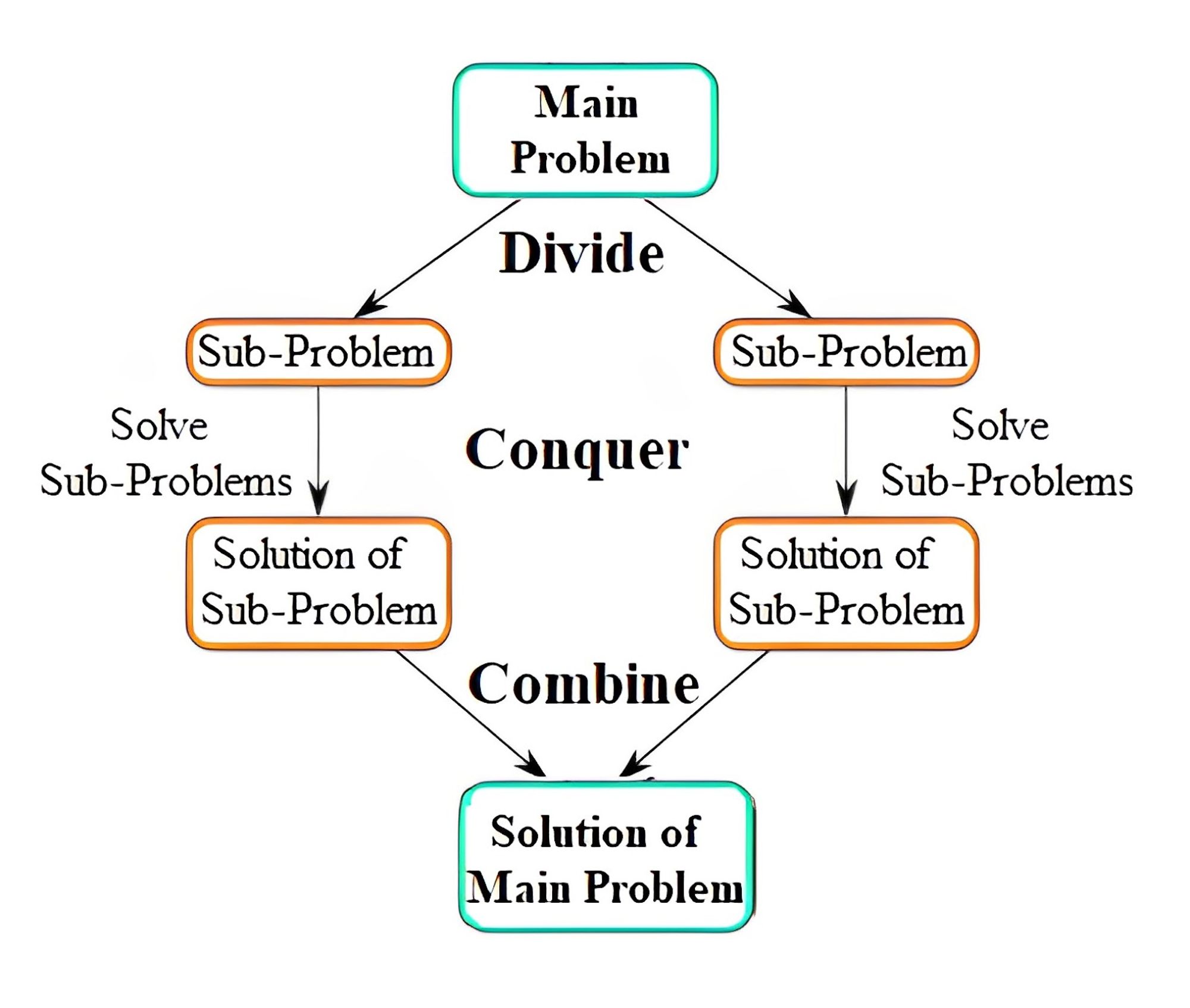
The divide-and-conquer paradigm is a problem-solving strategy that involves breaking down a problem into smaller subproblems, solving each subproblem independently, and then combining the solutions into a final solution for the original problem.
The basic steps of the divide-and-conquer paradigm are:
- Divide the problem into smaller subproblems.
- Conquer each subproblem by solving them recursively or iteratively.
- Combine the solutions of the subproblems into a solution for the original problem.
This strategy is often used in computer science and mathematics to solve complex problems efficiently.
It is especially useful for problems that can be broken down into smaller, independent subproblems, as it enables parallelization and can reduce the overall time complexity of the algorithm.
The divide-and-conquer paradigm can be a powerful tool for solving complex problems efficiently, but it requires careful consideration of how to divide the problem into subproblems and how to combine the solutions of those subproblems.
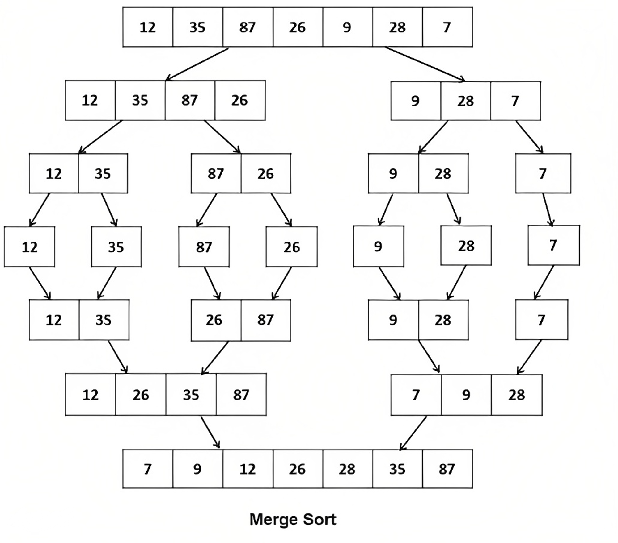
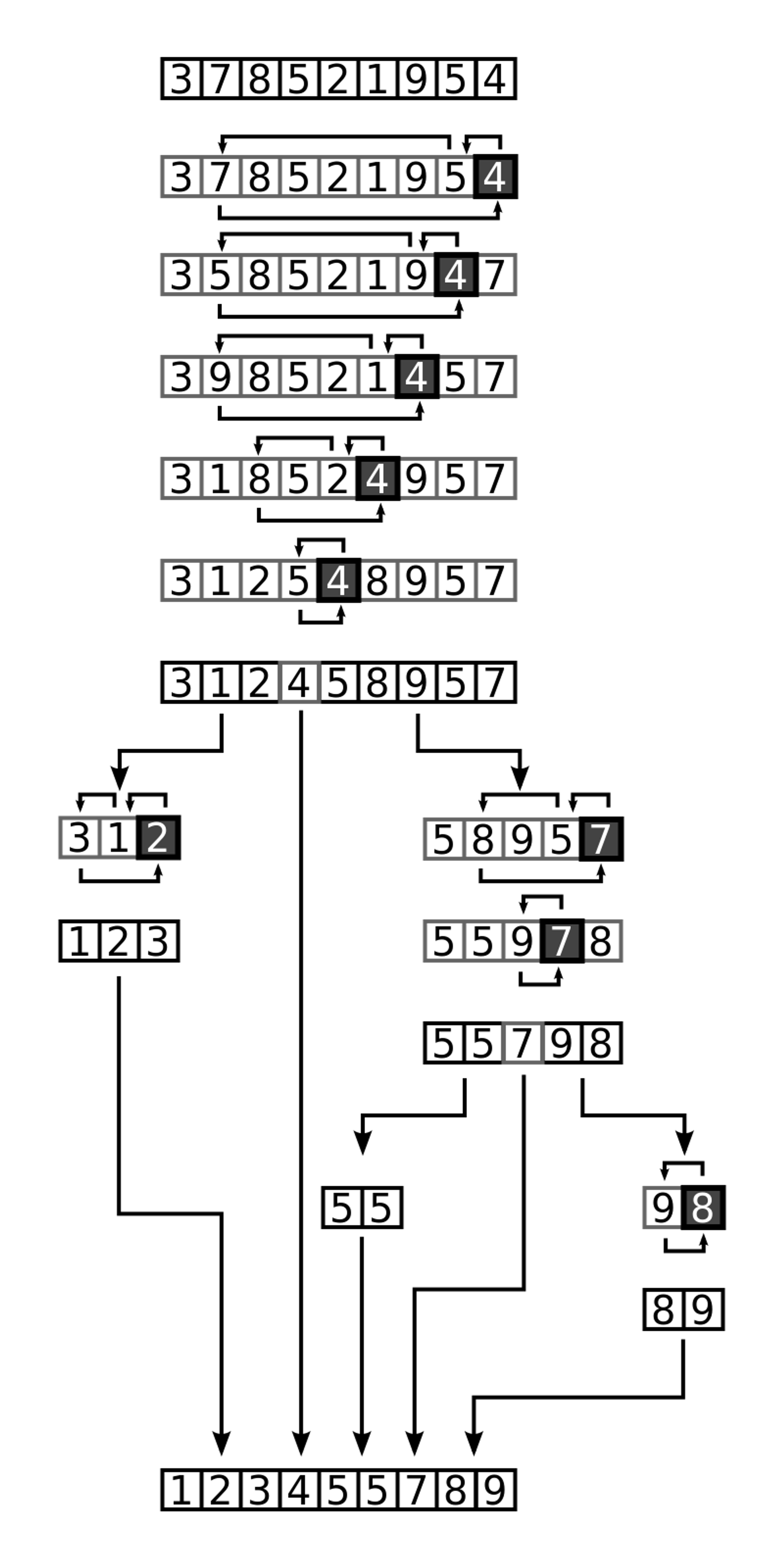
Merge Sort
Merge Sort is a popular sorting algorithm that follows the divide-and-conquer paradigm. It works by dividing the unsorted list into smaller sublists, sorting those sublists recursively, and then merging them back together into the final sorted list.
Here are the basic steps of the Merge Sort algorithm:
- Divide the unsorted list into two sublists of roughly equal size.
- Sort each of the sublists recursively by applying the same divide-and-conquer strategy.
- Merge the sorted sublists back together into one sorted list.
Merge Sort has a time complexity of O(n log n), making it more efficient than quadratic sorting algorithms like Bubble Sort, Selection Sort, and Insertion Sort for large datasets.
Additionally, Merge Sort is a stable sorting algorithm, meaning that it maintains the relative order of equal elements.
However, Merge Sort has a relatively high space complexity due to its use of additional memory during the merging process.
Implementation in JavaScript
const numbers = [99, 44, 6, 2, 1, 5, 63, 87, 283, 4, 0];

function mergeSort (array) {
    if (array.length === 1) {
      return array
    }
    // Split Array in into right and left
    const length = array.length;
    const middle = Math.floor(length / 2)
    const left = array.slice(0, middle)
    const right = array.slice(middle)
    // console.log('left:', left);
    // console.log('right:', right);

    return merge(
      mergeSort(left),
      mergeSort(right)
    )
  }

  function merge(left, right){
    const result = [];
    let leftIndex = 0;
    let rightIndex = 0;
    while(leftIndex < left.length &&
          rightIndex < right.length){
       if(left[leftIndex] < right[rightIndex]){
         result.push(left[leftIndex]);
         leftIndex++;
       } else{
         result.push(right[rightIndex]);
         rightIndex++
      }
    }
    // console.log(left, right)
    return result.concat(left.slice(leftIndex)).concat(right.slice(rightIndex));
  }

const answer = mergeSort(numbers);
console.log(answer);
Output
PS D:\Coding Playground> node playground2.js
[
    0,  1,  2,  4,  5, 6, 44, 63, 87, 99, 283
]
Quick Sort
Quick Sort is another popular sorting algorithm that uses the divide-and-conquer paradigm. It works by selecting a pivot element from the array, partitioning the array into two subarrays based on the pivot element, and then recursively sorting each subarray.
Here are the basic steps of the Quick Sort algorithm:
- Choose a pivot element from the array.
- Partition the array into two subarrays: one containing elements smaller than the pivot element, and one containing elements larger than the pivot element.
- Recursively apply Quick Sort to each subarray until the entire array is sorted.
Quick Sort has a time complexity of O(n log n) on average, making it one of the most efficient sorting algorithms for large datasets.
However, in the worst case (e.g., when the pivot element always selects the maximum or minimum element of the array), Quick Sort can have a time complexity of O(n^2).
This worst-case scenario can be avoided by selecting a good pivot element, such as the median or a random element.
Additionally, Quick Sort is an in-place sorting algorithm, meaning that it does not require additional memory beyond the original array.
Implementation in JavaScript
const numbers = [99, 44, 6, 2, 1, 5, 63, 87, 283, 4, 0];

function quickSort(array, left, right){
    const len = array.length;
    let pivot;
    let partitionIndex;

    if(left < right) {
      pivot = right;
      partitionIndex = partition(array, pivot, left, right);

      //sort left and right
      quickSort(array, left, partitionIndex - 1);
      quickSort(array, partitionIndex + 1, right);
    }
    return array;
  }

  function partition(array, pivot, left, right){
    let pivotValue = array[pivot];
    let partitionIndex = left;

    for(let i = left; i < right; i++) {
      if(array[i] < pivotValue){
        swap(array, i, partitionIndex);
        partitionIndex++;
      }
    }
    swap(array, right, partitionIndex);
    return partitionIndex;
  }

  function swap(array, firstIndex, secondIndex){
      var temp = array[firstIndex];
      array[firstIndex] = array[secondIndex];
      array[secondIndex] = temp;
  }

//Select first and last index as 2nd and 3rd parameters
quickSort(numbers, 0, numbers.length - 1);
console.log(numbers);
Output
PS D:\Coding Playground> node playground2.js
[
    0,  1,  2,  4,  5, 6, 44, 63, 87, 99, 283
]
Selecting a Sorting Algorithm
When selecting a sorting algorithm, it is important to consider various factors such as the size and distribution of the dataset, as well as the desired time and space complexity.
For large datasets with a relatively uniform distribution of values, Quick Sort and Merge Sort are generally good choices due to their efficient time complexity of O(n log n).
However, Quick Sort may perform poorly if the pivot element is not chosen carefully, resulting in a worst-case time complexity of O(n^2). Merge Sort is a stable sorting algorithm and has a space complexity of O(n).
Insertion Sort is a good choice for small datasets or nearly sorted data, with a best-case time complexity of O(n) when the data is already sorted. However, its worst-case time complexity of O(n^2) makes it less efficient for large datasets.
Selection Sort and Bubble Sort have a time complexity of O(n^2) and are generally less efficient than other sorting algorithms, especially for large datasets.
In summary, the choice of sorting algorithm should be based on careful consideration of various factors, including the size and distribution of the dataset, as well as the desired time and space complexity.
It is also important to test each sorting algorithm on the specific dataset to be sorted and compare their performance in terms of time and space complexity before making a final decision.
Comparison Sort Vs Non-Comparison Sort
Comparison Sort algorithms like Quick Sort, Merge Sort, Insertion Sort, Selection Sort, and Bubble Sort compare pairs of elements in the input array using comparison operators to determine their relative order.
Non-Comparison Sort algorithms like Counting Sort, Radix Sort, and Bucket Sort do not compare elements, but instead use other information about the elements to determine their correct positions in the sorted output.
Comparison Sort algorithms have a lower bound of O(n log n) time complexity, while Non-Comparison Sort algorithms can have a time complexity of O(n) in some cases.
Comparison Sort algorithms are more widely used and can handle a wider range of input data, but Non-Comparison Sort algorithms can be more efficient when their assumptions about the input data are met.
Nifty Snippet: What sort algorithm does the v8 engine's sort() method use?
In the V8 engine used by Google Chrome and Node.js, the Array.prototype.sort() method uses a hybrid sorting algorithm that combines Quick Sort and Insertion Sort.
The hybrid algorithm starts by using Quick Sort to partition the array into smaller subarrays, and once the subarrays become smaller than a certain threshold (usually 10-20 elements), it switches to Insertion Sort.
The reason for this hybrid approach is that Quick Sort is generally faster than Insertion Sort on large datasets, but Insertion Sort is faster than Quick Sort on small datasets or nearly sorted data.
By using a hybrid approach, the V8 engine can achieve good performance on a wide range of input data.
Searching Algorithms
Searching algorithms are important in computer science and programming because they enable efficient data retrieval and processing.
They provide time and resource efficiency, improve user experience, support better decision-making, and optimize the performance of more complex algorithms and data structures.
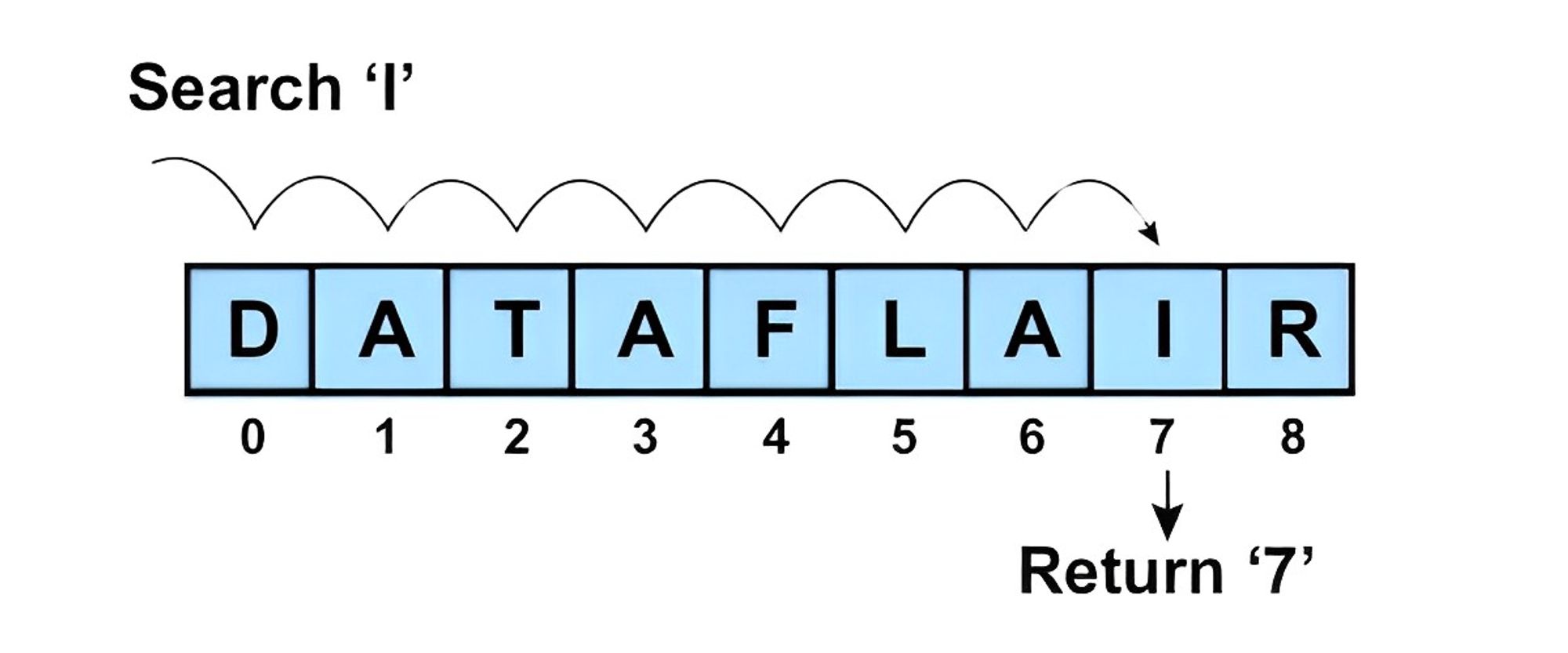
Linear Search
Linear search algorithm, also known as sequential search, is a simple searching algorithm that checks each element in a collection one by one until the desired element is found or the entire collection has been searched.
The steps involved in the linear search algorithm are as follows:
- Start at the beginning of the collection.
- Compare the first element to the desired element.
- If the elements match, the search is complete and the index of the element is returned.
- If the elements do not match, move to the next element in the collection and repeat steps 2 and 3.
- The entire collection has been searched and the element has not been found, return a message indicating that the element is not in the collection.
The time complexity of linear search is O(n), where n is the number of elements in the collection. This means that the time taken to search for an element increases linearly with the size of the collection.
Linear search is a simple and easy-to-understand algorithm, but it is not very efficient for large collections. It is best suited for small collections or for situations where the collection is unsorted or constantly changing.
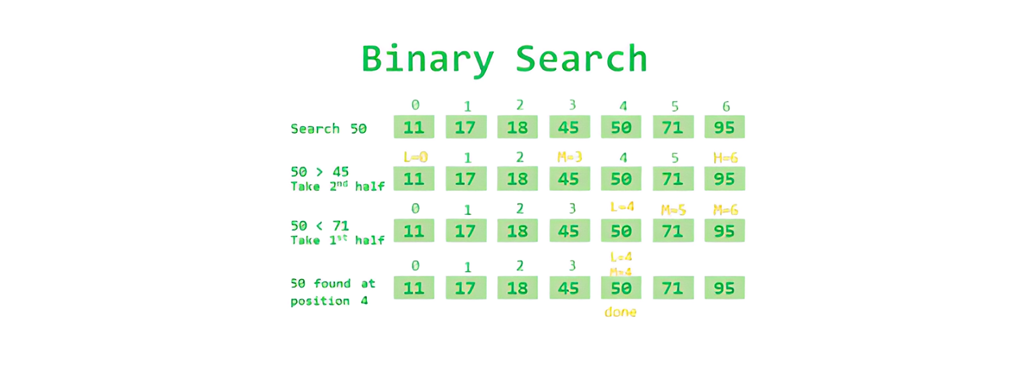
Binary Search
Binary search algorithm is a searching algorithm used for finding an element in a sorted collection. The algorithm works by repeatedly dividing the collection in half and checking if the desired element is in the left or right half.
The steps involved in the binary search algorithm are as follows:
- Start with the middle element of the collection.
- Compare the middle element to the desired element.
- If the middle element is equal to the desired element, the search is complete and the index of the element is returned.
- If the middle element is greater than the desired element, the search is conducted on the left half of the collection.
- If the middle element is less than the desired element, the search is conducted on the right half of the collection.
- Repeat steps 2-5 until the element is found or the search has been conducted on the entire collection.
The time complexity of binary search is O(log n), where n is the number of elements in the collection. This means that the time taken to search for an element increases logarithmically with the size of the collection.
Binary search is an efficient algorithm for searching in sorted collections, especially for large collections.
However, it requires the collection to be sorted before the search begins. If the collection is unsorted, a sorting algorithm must be used before binary search can be applied.
Traversal vs. Searching
Traversal involves visiting each element in a data structure and performing some operation on it, while search involves finding a specific element in a data structure based on some criteria.
Traversal is often used to process or analyze the data in a data structure, while searching algorithms are used to efficiently find the desired element.
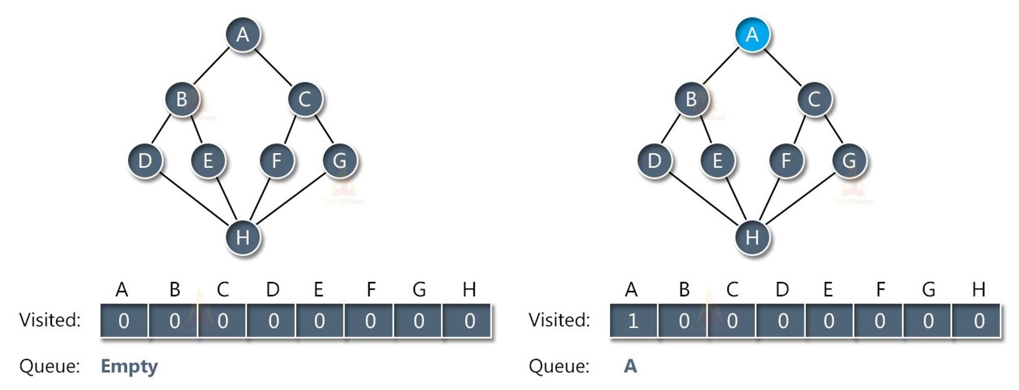
BFS
Breadth-First Search (BFS) is a traversal algorithm that starts at a specified node and explores all the neighboring nodes at the current level before moving on to the next level. It uses a queue data structure to keep track of the nodes to be visited next.
The steps involved in the BFS algorithm are as follows:
- Start at a specified node.
- Enqueue the node to a queue and mark it as visited.
- While the queue is not empty: a. Dequeue a node from the front of the queue. b. Visit the node and perform some operation on it. c. Enqueue all the neighboring nodes that have not been visited before and mark them as visited.
- Repeat step 3 until the queue is empty.
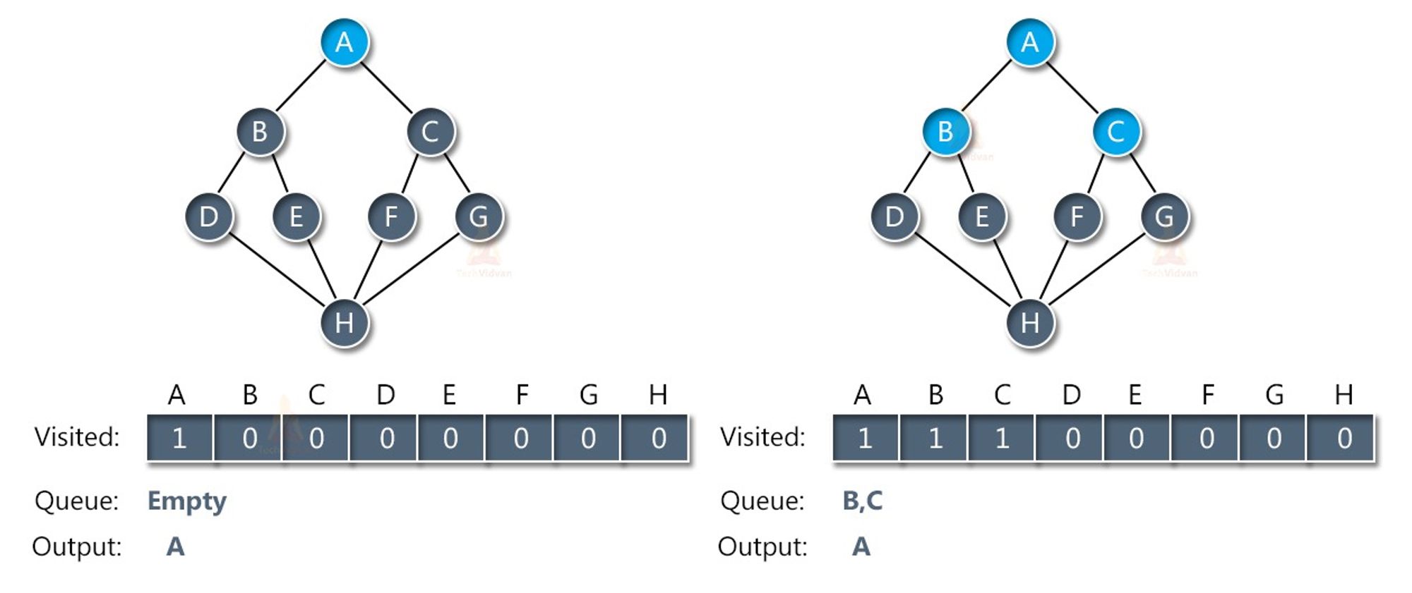
BFS visits all the nodes at each level before moving on to the next level. This ensures that the shortest path between two nodes in an unweighted graph is found. BFS can also be used to find the minimum number of steps required to reach a node from the starting node.
The time complexity of BFS is O(V+E), where V is the number of vertices and E is the number of edges in the graph. The space complexity of BFS is also O(V+E), as it needs to keep track of all the visited nodes and the nodes in the queue.
BFS is a useful algorithm for finding the shortest path in an unweighted graph, and for exploring all the nodes in a graph that are reachable from a starting node.
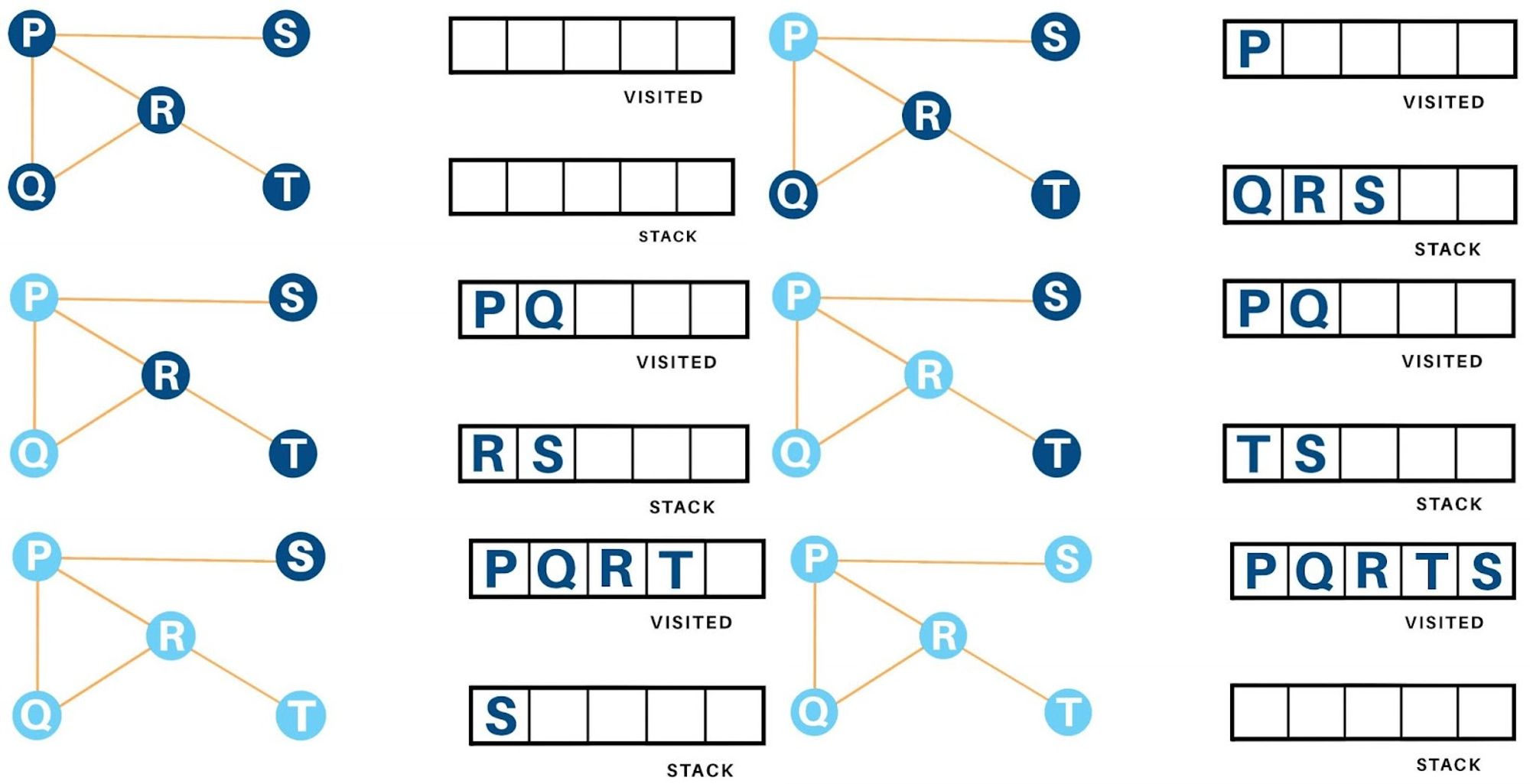
DFS
Depth-First Search (DFS) is a traversal algorithm that starts at a specified node and explores as far as possible along each branch before backtracking. It uses a stack data structure to keep track of the nodes to be visited next.
The steps involved in the DFS algorithm are as follows:
- Start at a specified node.
- Push the node to a stack and mark it as visited.
- While the stack is not empty:
- Pop a node from the top of the stack.
- Visit the node and perform some operation on it.
- Push all the neighboring nodes that have not been visited before to the stack and mark them as visited.
- Repeat step 3 until the queue is empty.
DFS explores all the nodes in a branch before backtracking to explore other branches. This makes it useful for exploring all the nodes in a graph and for detecting cycles in a graph. DFS can also be used to find a path between two nodes in a graph.
There are three types of DFS traversal:
- In-Order
- Pre-Order
- Post-Order
In-Order traversal visits the left subtree, then the current node, and then the right subtree.
Pre-Order traversal visits the current node, then the left subtree, and then the right subtree.
Post-Order traversal visits the left subtree, then the right subtree, and then the current node.
The time complexity of DFS is O(V+E), where V is the number of vertices and E is the number of edges in the graph. The space complexity of DFS is O(V), as it needs to keep track of all the visited nodes and the nodes in the stack.
DFS is a useful algorithm for exploring all the nodes in a graph and for detecting cycles in a graph. It can also be used to find a path between two nodes in a graph.
BFS vs. DFS
| BFS | DFS | |
|---|---|---|
| Approach | Explores level by level | Explores branch by branch |
| Data Structure | Uses a queue | Uses a stack or recursion |
| Memory Usage | Requires more memory | Requires less memory |
| Time Complexity | O(V+E) | O(V+E) |
| Use Cases | Shortest path in unweighted graph, reachable nodes from a starting node | Detecting cycles, exploring all nodes in a graph |
Note that while BFS and DFS have their own strengths and weaknesses, the actual performance of the algorithms may depend on the structure and size of the graph being traversed.
BFS Good at 😀:
- Shortest Path
- Closer Nodes
BFS Bad at 😒:
- More Memory
DFS Good at 😀:
- Less Memory
- Does Path Exist?
DFS Bad at 😒:
- Can Get Slow
Selecting a Searching Algorithm
Linear search is recommended for small, unsorted data or when the order of the elements does not matter. It is a simple algorithm that checks each element of the collection until the target element is found or the end of the collection is reached.
Linear search is easy to implement but can be inefficient for large collections since it has a time complexity of O(n), where n is the number of elements in the collection.
Binary search is recommended for sorted data, as it takes advantage of the sorted order and uses a divide-and-conquer approach to find the target element. It repeatedly divides the search interval in half until the target element is found or the search interval is empty.
Binary search has a time complexity of O(log n), which is much faster than linear search for large collections.
BFS (Breadth-First Search) is recommended for finding the shortest path or distance between two nodes in a graph or tree.
BFS explores all the nodes at the same level before moving to the next level. It uses a queue data structure to keep track of the nodes to be explored and has a time complexity of O(V+E), where V is the number of nodes and E is the number of edges in the graph.
DFS (Depth-First Search) is recommended for exploring all the nodes in a graph or tree. DFS explores as far as possible along each branch before backtracking. It uses a stack data structure to keep track of the nodes to be explored and has a time complexity of O(V+E), where V is the number of nodes and E is the number of edges in the graph.
In summary, the choice of the search algorithm depends on the properties of the data, the order of the elements, and the specific problem being solved. The time complexity of each algorithm should also be considered, as it can greatly impact the performance of the search.
Dijkstra and Bellman-Ford
Another two algorithms for finding the shortest path between two nodes in a graph are the Bellman-Ford and Dijkstra algorithms.
Bellman-Ford can handle graphs with negative edge weights, while Dijkstra cannot.
Bellman-Ford algorithm performs relaxation of all edges in the graph repeatedly until it finds the shortest path with a time complexity of O(VE), while Dijkstra algorithm maintains a priority queue of the next nodes to visit, with a time complexity of O((V+E)logV).
The choice between the two algorithms depends on the properties of the graph being searched.
If the graph has negative edge weights, Bellman-Ford should be used.
If the graph has only non-negative edge weights, Dijkstra may be faster for sparse graphs.
Negative Edge Weights
In graphs, an edge weight is a number assigned to an edge that represents a cost or benefit of traversing that edge.
Negative edge weights are when the assigned number is negative, which usually represents a cost or penalty associated with traversing the edge. Some algorithms for graph problems cannot handle negative edge weights, while others can.
Negative edge weights may make problems more complicated and require different algorithms or modifications to handle them.
Relaxation
Relaxation is the process of updating the estimated cost or distance to reach a node in a graph when a shorter path to that node is found.
It's a necessary step in algorithms that search for the shortest path in a graph, such as the Bellman-Ford algorithm.
Relaxation helps to find the shortest path by continuously updating the estimated distances until the shortest path is found.
Sparse Graphs
A sparse graph is a graph that has relatively few edges compared to the number of vertices it has. In other words, in a sparse graph, most pairs of vertices are not directly connected by an edge.
Sparse graphs are commonly found in real-world applications, such as social networks or transportation networks, where the number of connections or relationships between entities is much smaller than the total number of entities.
Because of their sparsity, some algorithms can be faster to execute on sparse graphs since they don't have to check as many edges.
Dynamic Programming
Dynamic programming is an optimization technique and a way to solve problems by breaking them down into smaller, simpler subproblems and storing the solutions to those subproblems.
By reusing those solutions instead of solving the same subproblems over and over again, we can solve the overall problem more efficiently.
Caching
Caching is a technique to store frequently accessed data or information in a temporary location called a cache. When the data is needed again, it can be retrieved much more quickly from the cache than from the original source.
This helps improve the speed and efficiency of accessing data, especially when dealing with large amounts of data or frequently accessed information.
Caching is used in many applications to improve overall system performance.
Memoization
Memoization, is a technique of caching or storing the results of expensive function calls and then reusing those results when the same function is called again with the same input parameters.
The idea behind memoization is to avoid repeating expensive calculations by storing the results of those calculations in memory. When the function is called again with the same input parameters, instead of recalculating the result, the function simply retrieves the previously calculated result from memory and returns it.
Caching vs. Memoization
Caching is used to store and retrieve frequently accessed data, while memoization is used to avoid repeating expensive calculations by storing the results of those calculations in memory for later use.
Example 1
// regular function that runs the entire process each time we call it
function addT080(n) {
    console. log( 'long time')
    return n + 80;
}

// an optimised function that returns the outcome of the previous input without repeating the entire process
function memoizedAddT080() {
    let cache = {};
    return function(n){
        if (n in cache) {
            return cache [n];
        } else {
            console. log( 'long time')
            cache [n] = n + 80;
            return cache [n]
        }
    }
}

const memoized = memoizedAddT080() ;
console.log('1', memoized(5))
console.log('2', memoized(5))
Output
PS D:\Coding Playground> node playground2.js
long time
1 85
2 85
Example 2
Let’s use another example to try to clarify the difference.
Suppose you have a web application that displays a list of products on a page. The product data is stored in a database. When a user requests the page, the application fetches the product data from the database and displays it on the page. If another user requests the same page, the application has to fetch the product data from the database again, which can be slow and inefficient.
To improve the performance of the application, you can use caching.
The first time the application fetches the product data from the database, it stores the data in a cache. If another user requests the same page, the application checks the cache first. If the data is in the cache, it can be retrieved much more quickly than if it had to be fetched from the database again.
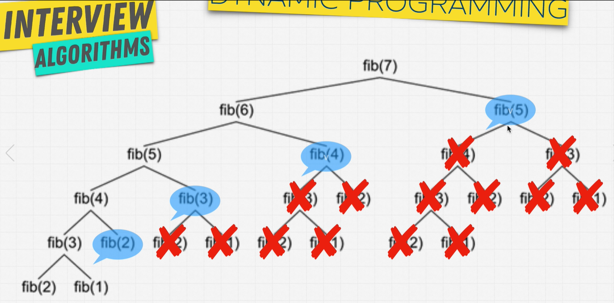
Now, suppose you have a function in your application that calculates the Fibonacci sequence. The calculation of the Fibonacci sequence is a computationally expensive task. If the function is called multiple times with the same input parameter, it would be inefficient to calculate the sequence each time.
To improve the performance of the function, you can use memoization.
The first time the function is called with a particular input parameter, it calculates the Fibonacci sequence and stores the result in memory. If the function is called again with the same input parameter, it retrieves the result from memory instead of recalculating the sequence.
When to use Dynamic Programming?
To find out if we need to use dynamic problem programming in a problem, We can use these steps.
- Can be divided into subproblem.
- Recursive Solution.
- Are there repetitive subproblems?
- Memoize subproblems.
And when you utilize it, you can ask your boss for a rise 🙂.

In general, dynamic programming is useful when a problem can be divided into smaller subproblems that can be solved independently, and the solutions to these subproblems can be combined to solve the overall problem.
By avoiding redundant calculations using memoization, dynamic programming can often provide significant performance improvements over other techniques for solving the same problem.
Credits
A huge thanks and credit goes to Zero To Mastery student, Khaled Elhannat!
This cheat sheet was created from his notes while taking the Master the Coding Interview: Data Structures and Algorithms course.