Getting Your Dataset To a Model in Production — Part 1

This is Part 1 of a series that walks you through all of the steps to build your own machine learning model starting from gathering data, all the way to deploying your model in production 🚀.

Hey everyone, Shubhamai here, I am a Machine Learning Engineer and a Machine Learning TA for Zero To Mastery. My interest and skills include ML, DL, Computer Vision, Natual Language Procession, and much more.

What’s the project?

So the project we are building is to take a plant’s leaf 🌿 from the user and predict is the leaf is healthy or not 😷. Using Tensorflow 2.0. Let’s get started!

In Part 1, we will discuss the following:

• Getting The Dataset

• Data Exploration

• Making The Training and Testing Dataset

• Making The Model

• Training & Testing

• Exporting The Model

Getting The Dataset (Fuel)⛽

I this section, we will discuss where we got the dataset and how you can get your own dataset for your own ideas and projects.

So the dataset we are using is from a Kaggle competition, Plant Pathology 2020 — FGVC7, to identify the category of foliar diseases in apple trees.

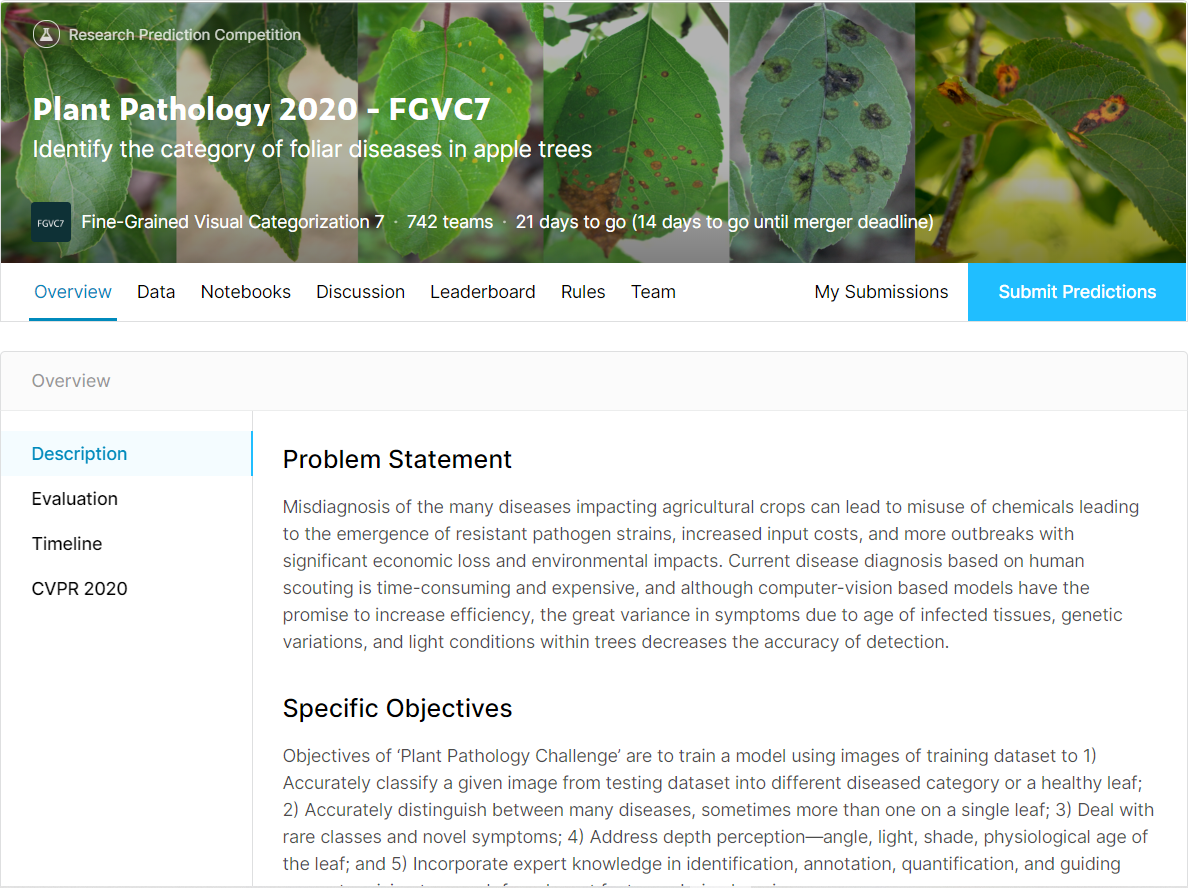
At the time of publishing this blog, this competition is still running and anyone can participate.

If you didn't know already, Kaggle is a home for data scientists and provides access to thousands of different dataset (and much more) so whenever you are searching for any dataset, try Kaggle first.

Data Exploration (Discovery)🧪

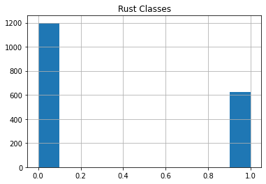
In this section, we will discuss the dataset (Exploratory Data Analysis) and target class distribution.

The Training Dataset looks something like this:

+-------------+---------+-------------------+------+------+
| image_id    | healthy | multiple_diseases | rust | scab |  
| Train_0.jpg | 0       | 1                 | 0    | 0    |  
| Train_1.jpg | 1       | 0                 | 0    | 0    |  
| Train_2.jpg | 0       | 0                 | 0    | 1    |  
+-------------+---------+-------------------+------+------+

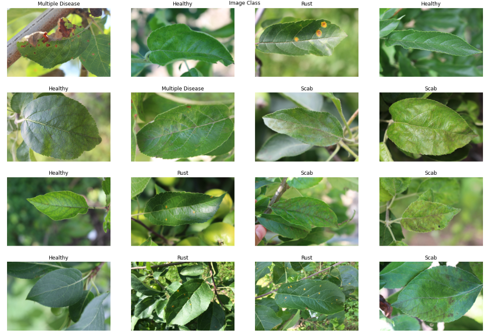
The training images are in another folder named images; there are four classes — healthy, multiple_diseases, rust, scab.

There is a total of 1,821 training images and 1,821 testing images. YES!

These are the images with their label class. The shape of images is (1365, 2048).

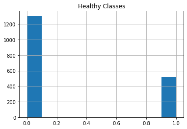
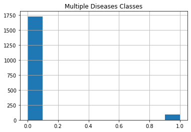
Data Distribution

Making The Training and Testing Dataset 🚂

To generate a batch of inputs and outputs for the model and to generate even MORE training data (Data Argumentation), we will use the Keras Data Generator ⚙

datagen = keras.preprocessing.image.ImageDataGenerator(
        rescale=1./255,  # Rescaling Image
        zca_whitening=False,  # apply ZCA whitening
        rotation_range=180,  # randomly rotate images in the range (degrees, 0 to 180)
        zoom_range = 0.15, # Randomly zoom image 
        width_shift_range=0.15,  # randomly shift images horizontally (fraction of total width)
        height_shift_range=0.15,  # randomly shift images vertically (fraction of total height)
        horizontal_flip=True,  # randomly flip images
        vertical_flip=True)  # randomly flip images

How Keras Generators Works

Keras Generator generates a Batch of Inputs and Outputs while training the model. The advantages of Keras Generators are:

1. They use very little memory

2. They offer Data Argumentation (a way to generate more training data) by:

   • Randomly flipping images horizontally or vertically
   • Randomly zooming and rotating the images
   • Randomly shifting the image (horizontally or vertically)
   • And much more…

3. They make it very easy to read image data and making inputs and outputs for the model

Fitting to Training Data

train_generator = datagen.flow_from_dataframe(dataset, 
                    directory='/kaggle/input/plant-pathology-2020-fgvc7/images/',
                    x_col='image_id',
                    y_col=['healthy', 'multiple_diseases', 'rust', 'scab'] , 
                    target_size=(512, 512), 
                    class_mode='raw',
                    batch_size=8, shuffle=False)

We read the image from the /image folder and the corresponding label of the images from getting from x_col='image_id'.

Resize the image to (512, 512), and the rest is pretty normal.

Making the Model (…)

In this section, we will make our Keras Model for training, and see the architecture of our model.

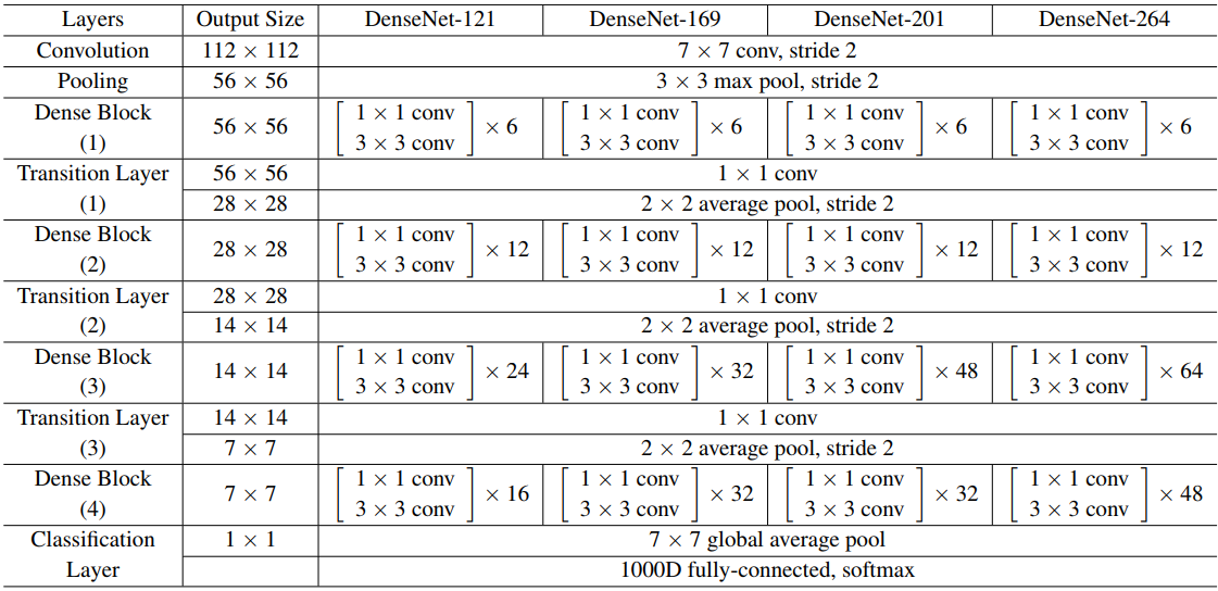
I've experimented with many models, Xception, DenseNet121, InceptionResNetV2, etc. After lots of experimentation (training different models), days of GPU, I've finally come to this point:

Ultimately, after this experimentation, I found that the combination of Xception and DenseNet121 (Ensembling Models) is performing best of all.

Architecture of networks

• Xception

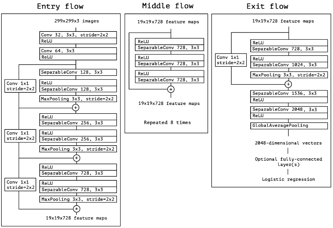
• DenseNet121

Ensembled Network

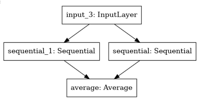
• The input layer is where the image comes

• The sequestion_1 & sequential are Xception and DenseNet121 with added GlobalAveragePooling2D and output layer in both networks

• The average layer takes the output from Xception and DenseNet121 and averages them

🥁🥁🥁... here is the code!

xception_model = tf.keras.models.Sequential([
tf.keras.applications.xception.Xception(include_top=False, weights='imagenet', input_shape=(512, 512, 3)),
 tf.keras.layers.GlobalAveragePooling2D(),
tf.keras.layers.Dense(4,activation='softmax')
])
xception_model.compile(optimizer='adam', loss='categorical_crossentropy', metrics=['accuracy'])

densenet_model = tf.keras.models.Sequential([
    tf.keras.applications.densenet.DenseNet121(include_top=False, weights='imagenet',input_shape=(512, 512, 3)),
   tf.keras.layers.GlobalAveragePooling2D(),
   tf.keras.layers.Dense(4,activation='softmax')
])
densenet_model.compile(optimizer='adam', loss='categorical_crossentropy', metrics=['accuracy'])

inputs = tf.keras.Input(shape=(512, 512, 3))

xception_output = xception_model(inputs)
densenet_output = densenet_model(inputs)

outputs = tf.keras.layers.average([densenet_output, xception_output])

model = tf.keras.Model(inputs=inputs, outputs=outputs)
model.compile(optimizer='adam', loss='categorical_crossentropy', metrics=['accuracy'])

Training The Model (Rest Time)

In this section, we will set LearningRateScheduler for our model and then train it, check the results and test it.

LearningRateScheduler

Learning rate in very important hyperparameter in Deep Learning. It calculates how much to change the model weights after getting the estimated error while training.

• Too low of a learning rate can slow down the learning process of the model and will take a much longer time to converge to optimal weights

• Too high of a learning rate can make the training process unstable

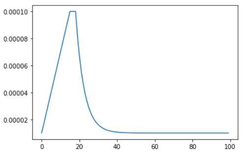
LR_START = 0.00001
LR_MAX = 0.0001 
LR_MIN = 0.00001
LR_RAMPUP_EPOCHS = 15
LR_SUSTAIN_EPOCHS = 3
LR_EXP_DECAY = .8
EPOCHS = 100

def lrfn(epoch):
    if epoch < LR_RAMPUP_EPOCHS:
        lr = (LR_MAX - LR_START) / LR_RAMPUP_EPOCHS * epoch + LR_START
    elif epoch < LR_RAMPUP_EPOCHS + LR_SUSTAIN_EPOCHS:
        lr = LR_MAX
    else:
        lr = (LR_MAX - LR_MIN) * LR_EXP_DECAY**(epoch - LR_RAMPUP_EPOCHS - LR_SUSTAIN_EPOCHS) + LR_MIN
    return lr

lr_callback = tf.keras.callbacks.LearningRateScheduler(lrfn, verbose=True)

rng = [i for i in range(EPOCHS)]
y = [lrfn(x) for x in rng]
plt.plot(rng, y)
print("Learning rate schedule: {:.3g} to {:.3g} to {:.3g}".format(y[0], max(y), y[-1]))

MODEL TRAINING

RESULTS

After ~8 HOURS of Model training.

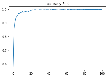
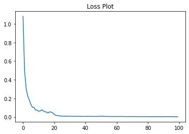
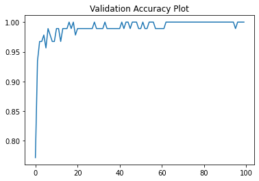
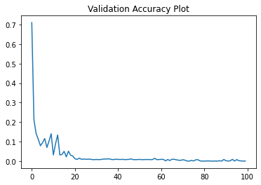
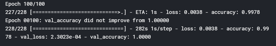
The performance is pretty amazing (if I do say so myself!).

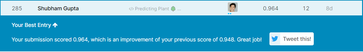
After predicting the testing dataset and submitting it to the competition… 😱

Exporting The Model

In this section, we will save our model architecture and model weights into a .h5 file extension (we will need this in the next section).

model.save('model.h5') # Saving Modle Weights with Architectues

model.save_weights('weights.h5') # Just Saving Model Weights 

Done... easy right?

Things Learned (MOST IMPORTANT)

• Ensembling Model (Always)

• Lookout for OVERFITTING

• Combination of Xception and Densenet121 (to try in future again)

If you want to see the full code and try it yourself, you can access the code here(upvote if you like it 😁).

Part 2?!?

In Part 2, we will solve this together…

Final Thoughts

Project Idea 💡

Given the entire world is dealing with COVID-19 🦠, why not try and contribute as a Machine Learning Engineer? YES!

The purpose of this particular project is to classify X-Ray images as COVID-19, Pneumonia, and Normal. Pretty interesting, isn't it?

There are many datasets out there, but these are some of the popular ones:

• COVID-19 Xray Dataset (recommended)

• COVID-19 image data collection

• Chest Xray Images PNEUMONIA and COVID-19

Try these dataset, build models and deploy them (and we'll learn deployment in part 2). Once you've built your model, share it with me, I love seeing projects by different people 😀

I hope you like this post. Let me know what else you are interested to see in the next post, or if there are any corrections or improvements. See you in the next post!